| Issue |
J. Eur. Opt. Society-Rapid Publ.
Volume 21, Number 1, 2025
|
|
|---|---|---|
| Article Number | 29 | |
| Number of page(s) | 7 | |
| DOI | https://doi.org/10.1051/jeos/2025024 | |
| Published online | 27 June 2025 | |
Research Article
Interpretation of three-dimensional polarization states through the smart decomposition of the polarization matrix
1
Group of Photonic Technologies, University of Zaragoza, Pedro Cerbuna 12, 50009, Zaragoza, Spain
2
Center for Photonics Sciences, University of Eastern Finland, PO Box 111, FI-80101 Joensuu, Finland
* Corresponding author: This email address is being protected from spambots. You need JavaScript enabled to view it.
Received:
24
April
2025
Accepted:
14
May
2025
Abstract
A complete description of a three-dimensional (3D) polarization state is provided by the two most significant eigenstates of the polarization matrix, together with the two indices of polarimetric purity. By means of the so-called smart decomposition, such information can be arranged to represent the state as a combination of two components, one partially polarized (active component) and one unpolarized. Contrary to what happens for two-dimensional (2D) polarization states (with the electric field fluctuating within a fixed plane), whose active component is constituted by a single totally polarized state, in the general case of 3D polarization states the active component is given by a weighted incoherent composition of the two above-mentioned eigenstates. We show that a detailed description of the intensity and spin anisotropies is encompassed by the active component of the state, which admits a simple interpretation and geometric representation. In addition, it is found that the degree of nonregularity can be viewed as a distance of the state to a regular state.
Key words: Polarization / Nonparaxial light / Smart decomposition / Nonregular polarization states
© The Author(s), published by EDP Sciences, 2025
 This is an Open Access article distributed under the terms of the Creative Commons Attribution License (https://creativecommons.org/licenses/by/4.0), which permits unrestricted use, distribution, and reproduction in any medium, provided the original work is properly cited.
1 Introduction
The polarization properties of an electromagnetic wave at a given point in space are represented by the associated 3 × 3 polarization matrix (also called coherency matrix). Leaving aside the particular well-known case of partially polarized states whose electric field fluctuates in a fixed plane (hereafter called two-dimensional (2D) polarization states), recent advances in the study and control of light related to near-field phenomena, tightly focused beams, and nanotechnology in general, have stimulated much interest in true three-dimensional (3D) polarization states [1–13]. Paralleling this progress, interpretations of the polarization matrix from algebraic, statistical, and geometrical points of view have been dealt with in a number of contributions from both theoretical and applied perspectives [14–28]. While the polarization matrix describes local polarization effects, the 3D polarization features of spatially distributed (random and deterministic) fields have also been actively studied [29–37].
In this work, the frame for the physical interpretation of genuine 3D polarization states is set by the so-called smart decomposition, which expresses the 3 × 3 polarization matrix as an incoherent composition of two totally polarized states (called pure states) and a totally unpolarized 3D state [21, 38]. This approach provides a new view on certain properties, like the degree of nonregularity [39], obtained previously through other procedures. In general, the analysis relies on the fact that the unpolarized component does not carry any information on the shape of the polarization object, composed of the intensity ellipsoid and the spin vector of the state [17, 27, 40]. The component which is not unpolarized, hereafter called the active component, depends on the specific configuration of the pair of eigenstates associated with the largest eigenvalues of the polarization matrix, and it determines the intensity and spin anisotropies of the polarization state. This means that, up to a scale factor fixed by the relative weight of the unpolarized component, all polarization descriptors, including the nine 3D Stokes parameters, the spin vector, the degree of nonregularity, etc., are provided by the active component.
The structure and main points of the work are as follows. Section 2 is devoted to introducing the theoretical framework necessary to describe the original results presented in Sections 3–5, which include the definition of the active component of a polarization state as a representative of the intensity and spin anisotropies in a simple and condensed manner. The smart decomposition (without using this name) was introduced for the first time in [21] and then also described in [38]; nevertheless, some aspects like the indices of polarimetric purity (IPP) of the active component and their relations to those of the whole state are introduced here for the first time, allowing a deeper insight into the sources of the polarization properties of the state. The presented approach also allows us to interpret any given 3D polarization state in terms of its two more significant eigenstates (those with larger associated eigenvalues). In addition, the concept of nonregularity is revisited and interpreted as a distance of the state to a regular state as well as in terms of the spin of the discriminating component.
2 3D and 2D polarization states
In the most general 3D representation, the second-order polarization properties of random (stationary) light at a given point in space are fully characterized by the corresponding 3 × 3 polarization matrix (1)where εx(t), εy(t), εz(t) are the analytic signals [41] of the electric field components [14, 42] with respect to the given Cartesian reference frame XYZ [21]. In addition, the asterisk indicates complex conjugation and 〈…〉 represents time averaging. The polarization matrix can be expressed as
  in terms of the intensity I = trR (tr representing the trace) and the so-called polarization density matrix
  .
.
The matrix  is fully characterized mathematically by its Hermiticity and positive semidefiniteness together with the normalization condition
  . It can be expressed as
 (2)where diag indicates a diagonal matrix,
  with
with  are the eigenvalues of
  , and U is a unitary matrix whose columns
  are the three-component Jones vectors of the corresponding orthonormal eigenstates [43]. The eigenvalues specify the structure of polarimetric purity-randomness, which is characterized through the pair of indices of polarimetric purity (IPP) [16, 19, 44]
 (3)
(3)
The IPP are independent of intensity and satisfy the nested inequalities 0 ≤ P1 ≤ P2 ≤ 1. The eigenvalues of R are given by  (i = 1, 2, 3).
In the particular case of 2D states, the reference axis Z can be taken orthogonal to the well-defined polarization plane XY, so that the polarization matrix can straightforwardly be reduced to its conventional 2 × 2 form (4)where s0, s1, s2, s3 are the traditional Stokes parameters of a 2D field. Above, despite that common experiments or arrangements on 2D polarization states do not necessitate to consider explicitly the third axis Z, its existence is nevertheless implicitly assumed. In fact, the representation of a 2D state can be referenced with respect to arbitrary 3D reference frames, in which case nonzero components associated with the Z axis appear [45]. The transformation of the original reference axes XYZ to the new Cartesian ones X′Y′Z′ is performed through a rotation represented by the corresponding orthogonal matrix Q. The polarization matrix
  expressing the state R
2D in the new reference frame is then given by
expressing the state R
2D in the new reference frame is then given by![Mathematical equation: $$ {\mathbf{R}}_{2D}^\mathrm{\prime}=\mathbf{Q}\left[\frac{1}{2}\left(\begin{array}{ccc}{s}_0+{s}_1& {s}_2-i{s}_3& 0\\ {s}_2+i{s}_3& {s}_0-{s}_1& 0\\ 0& 0& 0\end{array}\right)\right]{\mathbf{Q}}^{\mathrm{T}}, $$](/articles/jeos/full_html/2025/01/jeos20250030/jeos20250030-eq15.gif) (5)where the superscript T indicates transpose. Explicit expressions for the above 3D representation of the polarization matrix of a 2D state can be found in [45]. States that cannot be represented as in equation (5) are called genuine 3D states because they necessarily require a 3D representation, i.e., the intensities of the three components of the fluctuating electric field are nonzero regardless of the reference frame taken to represent the corresponding polarization matrix.
(5)where the superscript T indicates transpose. Explicit expressions for the above 3D representation of the polarization matrix of a 2D state can be found in [45]. States that cannot be represented as in equation (5) are called genuine 3D states because they necessarily require a 3D representation, i.e., the intensities of the three components of the fluctuating electric field are nonzero regardless of the reference frame taken to represent the corresponding polarization matrix.
Let us now recall that the term regular has been coined to refer to those 3D states that can be represented as an incoherent composition of a 2D polarization state (pure or not) and a 3D unpolarized state [39] (see Fig. 1). It has been shown that such a property is not general but particular; 3D polarization states are generally nonregular [39]. Thus, regular states are those that can be expressed as![Mathematical equation: $$ \begin{array}{l}\mathbf{R}=\mathbf{Q}\left[\frac{1}{2}\left(\begin{array}{ccc}{s}_0+{s}_1& {s}_2-i{s}_3& 0\\ {s}_2+i{s}_3& {s}_0-{s}_1& 0\\ 0& 0& 0\end{array}\right)\right]{\mathbf{Q}}^{\mathrm{T}}+{\mathbf{R}}_{u-3D},\\ \left[{\mathbf{R}}_{u-3D}={I}_u{\mathbf{I}}_3/3\right],\\ \end{array} $$](/articles/jeos/full_html/2025/01/jeos20250030/jeos20250030-eq16.gif) (6)where I
3 is the 3 × 3 identity matrix and R
u−3D is the polarization matrix of a 3D unpolarized state with intensity Iu, which is invariant under arbitrary rotations of the Cartesian reference frame, i.e., QR
u−3D
Q
T = R
u−3D. Accordingly, through an appropriate choice of the reference frame, regular states can be represented as
(6)where I
3 is the 3 × 3 identity matrix and R
u−3D is the polarization matrix of a 3D unpolarized state with intensity Iu, which is invariant under arbitrary rotations of the Cartesian reference frame, i.e., QR
u−3D
Q
T = R
u−3D. Accordingly, through an appropriate choice of the reference frame, regular states can be represented as (7)
(7)
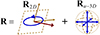 |
Figure 1 3D polarization states R that can be decomposed into a 2D state R 2D and a fully unpolarized 3D state R u−3D are called regular, and nonregular otherwise. |
On the other hand, 3D states that cannot be represented as in equation (7) are nonregular.
A simplified and meaningful view of the polarization matrix of a generic polarization state in the 3D space (regardless of whether it is pure, 2D, regular, or nonregular) is given by its intrinsic representation [21] (8)with the intensity-normalized eigenvalues of the real part Re(R) satisfying
  and
and  The orthogonal rotation matrix Q
O diagonalizes Re(R) [17, 21], viz.,
The orthogonal rotation matrix Q
O diagonalizes Re(R) [17, 21], viz., (9)
(9)
Note that the intrinsic polarization matrix R
O represents the same state as R, but with respect to the so-called intrinsic reference frame XO
YO
ZO instead of XYZ for R. A genuine property of R
O is that its off-diagonal elements are purely imaginary and determine the spin vector  of the state [17, 21, 40].
The quantities involved in R
O are directly related to the six so-called intrinsic Stokes parameters of the state  [21, 27, 46]. The degree of linear polarization Pl and the degree of directionality Pd (a measure of the stability of the plane containing the polarization ellipse) are defined analogously to the IPP by replacing the eigenvalues
  of the polarization density matrix with the intensity-normalized principal intensities
  , i.e.,
 (10)which obey 0 ≤ Pl ≤ Pd ≤ 1. Moreover, the degree of circular polarization is given by
  [21, 47], where
  . It is invariant under rotations of the Cartesian reference frame and consequently
  , with
  being the intensity-normalized spin vector in the arbitrary reference frame XYZ. Note that, as occurs with the IPP, the descriptors Pl, Pd, and Pc are intensity-independent.
For further analyses, we also mention the geometric representation of the polarization state in terms of the polarization object, constituted by the intensity ellipsoid (whose semiaxes are the principal intensities) together with the spin vector [27]. Other parameters that will be useful are the so-called degree of elliptical purity [44] (11)and the degree of polarimetric purity [16, 46]
 (12)
(12)
Note that in general P1 ≤ Pe and P2 ≤ Pd [38], while the above dual expression for P3D implies the equality 
3 Smart decomposition
The representation of the polarization density matrix in equation (2) implies the so-called spectral decomposition (13)where
  Here ⊗ stands for the Kronecker product, the dagger indicates conjugate transpose, and the subscript p emphasizes that the state is pure. The spectral decomposition can be rearranged into the smart decomposition [38]
 (14)which in terms of the two IPP takes the interesting form [21]
 (15)
(15)
Equivalently we may write (16)where the active component
 (17)encompasses all the information on the intensity and spin anisotropies of the polarization state up to the scale coefficient P2.
Equation (15) indicates that  is fully determined by the pair of IPP, which regulate the coefficients of the smart decomposition, together with the two first eigenvectors
  and
and  , associated with the two more significant eigenstates specifying
  and
and  , respectively. The third eigenstate
  does not appear explicitly in the smart decomposition because it is fixed by the pair (
 ). In view of equations (13) and (14) the respective portions
  and
and  have been subtracted from the two more significant pure components in order to group them with
  , thus building the fully unpolarized component
  , which in turn has a fully isotropic structure and therefore does not carry any information on polarimetric anisotropies.
Consequently, according to equation (16), any polarization state (3D in general) can be interpreted as a superposition of (a) a partially polarized state (the active component), given by the incoherent composition of the two pure components  and
and  with respective weights (P1 + P2)/2 and (P2 − P1)/2, which in turn are determined by the two eigenstates
  and
and  of more significant eigenvalues; and (b) a fully unpolarized 3D state weighted by 1 – P2. Notice that the weight affecting R
p1 is never smaller than that of R
p2.
of more significant eigenvalues; and (b) a fully unpolarized 3D state weighted by 1 – P2. Notice that the weight affecting R
p1 is never smaller than that of R
p2.
To further understand the smart decomposition, it is worth comparing it with the so-called characteristic decomposition [19, 44] (18)where the middle term, given by
  and called the discriminating component [48, 49], consists of an equiprobable incoherent mixture of the two first eigenstates. Naturally, the active parts of the smart and characteristic decompositions coincide but are expressed through respective decompositions. The smart decomposition is illustrated in Figure 2 for a generic configuration.
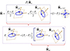 |
Figure 2 The active component of a polarization state admits an interpretation either as an incoherent composition of two pure states, the first two eigenstates, or equivalently as an incoherent combination of the pure and discriminating components of the state. |
From the very definition of the active component, its characteristic decomposition has the form (19)
(19)
Therefore, the IPP of  , denoted by Pa1 and Pa2, which obviously coincide with those of R
a, are proportional to those of R via the coefficient 1/P2 ≥ 1, i.e., Pa1 = P1/P2 ≥ P1 and Pa2 = 1 ≥ P2. Consequently, the polarization object of the active component
, denoted by Pa1 and Pa2, which obviously coincide with those of R
a, are proportional to those of R via the coefficient 1/P2 ≥ 1, i.e., Pa1 = P1/P2 ≥ P1 and Pa2 = 1 ≥ P2. Consequently, the polarization object of the active component  , whose principal intensities and intrinsic spin vector are denoted as
  and
and  , coincides with that of
  except for the scale coefficient 1/P2 as illustrated in Figure 3.
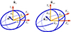 |
Figure 3 The shapes and orientations of the polarization objects of the polarization matrix and its active component coincide but differ by a scale coefficient 1/P2 ≥ 1 as |


4 Configurations of the active component
An algebraic and geometric representation of all possible configuration sets of 3D orthonormal states was described in [43], which can be applied to the three orthonormal eigenstates  of
of  . As an example, a representative family of configurations of the triad of eigenstates is shown in Figure 4, where the intrinsic axes X1, Y1, Z1 of the first eigenstate are taken as the reference frame for the three eigenstates. All families share the property that, when the polarization planes of two eigenstates coincide, the third one corresponds to a linearly polarized state along the direction orthogonal to the said planes [43].
 |
Figure 4 Example of a family of configurations of the polarization eigenstates |


Since a fully unpolarized state R
u−3D lacks spin, the smart decomposition shows that the normalized spin vector  can be expressed as a weighted sum of the normalized spin vectors
  and
and  related to the two first eigenvectors
  and
and  ,
, (20)so that
  . We note that regular states are characterized by the fact that the eigenstates
  and
and  have opposite normalized spin vectors,
  . Consequently, the normalized spin vector of a regular state is given by
  , in accordance with the fact that the entire spin originates from the pure component of the characteristic decomposition.
5 Interpretation of nonregularity
For a regular state the discriminating component  is necessarily a 2D unpolarized state, while otherwise the state is nonregular. Since
  , and hence nonregularity, depends on the relative configurations of the two more significant eigenstates
  and
and  , nonregularity has a direct relation to the smart decomposition. In particular, from the analysis performed in Sections 2 and 3, it follows that a polarization state R is regular if and only if any of the following conditions holds: (a)
  (i.e.,
  is a real-valued matrix); (b) the angle θ2 subtended by the polarization planes of the eigenstates
  and
and  is zero (see Fig. 4); (c)
  has zero spin; (d)
  ; (e)
; (e)  ; (f) the third eigenstate
  of R is linearly polarized; (g) P1 = Pe, and (h) P2 = Pd. In addition, we stress that states satisfying
  (thus susceptible to being represented as incoherent superpositions of linearly polarized states) are always regular. Conditions (a) to (f) follow directly from the analyses performed above. Property (g) comes from the fact that Pd is defined in equation (10) from the ordered eigenvalues
  of Re(R) while P2 is defined in equation (3) from the ordered eigenvalues
  of
of  , so that necessarily
  and thus P2 ≥ Pd, with the equality P2 = Pd corresponding, uniquely, to regular states
  . These considerations together with equation (12) imply P1 ≤ Pe and property (h) [38].
As shown in [38, 39], in its own intrinsic reference frame XmO
YmO
ZmO, the discriminating component adopts the simple form (21)where −π/4 ≤ χm3 ≤ π/4 is the ellipticity angle of the third eigenstate
  of
of  . It is remarkable that regular states are characterized by χm3 = 0, showing that R is regular if and only if
  represents a linearly polarized state. This property is similar to, but different from, condition (f) described above (which refers to
  instead of
  ).
).
A proper way to quantify the nonregularity of  is to consider the distance from
  to
to  . Note that, since R
m has been defined under the convention λ1 ≥ λ2 ≥ λ3, it necessarily takes the form R
u−2D = (I/2)diag (1, 1, 0) for regular states (that is, the regular form of R
m corresponds to an unpolarized 2D state whose electric field fluctuates in the common polarization planes of the eigenstates
. Note that, since R
m has been defined under the convention λ1 ≥ λ2 ≥ λ3, it necessarily takes the form R
u−2D = (I/2)diag (1, 1, 0) for regular states (that is, the regular form of R
m corresponds to an unpolarized 2D state whose electric field fluctuates in the common polarization planes of the eigenstates  and
and  ). On employing the Frobenius norm, which is invariant under orthogonal similarity transformations (i.e., rotations of the reference frame), we obtain
 (22)where |χm3| ≤ π/4 implies
  . By normalizing this squared distance in order to take values from 0 (regularity) to 1 (maximal nonregularity of
  ) we define the degree of nonregularity of
  as
as (23)which coincides with the definition introduced previously in terms of the smallest eigenvalue
  of
of  [39]. Now, by taking into account the relative weight (P2 – P1) of the discriminating component in the characteristic decomposition of equation (18), the degree of nonregularity of the state R is given by
 (24)
(24)
Thus, even though the state  does not determine the remaining pair of eigenstates
  and
and  of R
m, the constituents of the active component of R
m, its ellipticity angle governs the degree of nonregularity of the state R as seen from equation (24). Conversely, since the orthonormal vectors
of R
m, the constituents of the active component of R
m, its ellipticity angle governs the degree of nonregularity of the state R as seen from equation (24). Conversely, since the orthonormal vectors  constitute the columns of the unitary matrix that diagonalizes
  , the pair
  fixes completely
  .
.
Furthermore, equation (21) shows that the absolute value of the intensity-normalized spin vector  of
of  , which is invariant under arbitrary rotations of the reference frame, is given by
 (25)which establishes the link between the nonregularity of R and
  via the angular parameter χm3. More precisely, as indicated above, the minimal value
  is a genuine property of regular states (χm3 = 0), while the maximum
  corresponds, uniquely, to so-called perfect nonregular states (|χm3| = π/4) [39]. It is remarkable that, contrary to the spin vector of a regular state whose direction is normal to the plane containing the two largest principal intensities, the vector
  exhibits transversal character in the sense that it lies along the axis XmO defined by the largest principal intensity of
  . The analysis of the spin vector of R as the weighted sum of the spin vectors of the pure and discriminating components of R is studied in [48].
6 Conclusions
A simplified and meaningful interpretation of 3D polarization states can be attained from the (orthonormal) eigenstates  and
and  of R associated with the two largest eigenvalues, together with the indices of polarimetric purity. Such information determines the active component of R, which is introduced from the smart decomposition and provides a complete description of the spin and intensity anisotropies of the polarization state. Furthermore, the specific configuration of the pair (
 ) arbitrates the nonregularity and the transverse component of the spin vector by means of a single angular parameter. The concept of nonregularity was revisited in light of the indicated results and interpreted in terms of a distance of the state to a regular one.
Funding
Research Council of Finland (349396, 354918, PREIN 346518).
Conflicts of interest
The authors have nothing to disclose.
Data availability statement
No data were generated in this study.
Author contribution statement
J.J.G. developed the theory with contributions from T.S., A.N., and A.T.F. Original draft was prepared by J.J.G. and further edited by T.S., A.N., and A.T.F.
References
- Setälä T, Shevchenko A, Kaivola M, Friberg AT, Degree of polarization for optical near fields, Phys. Rev E 66, 016615 (2002). [Google Scholar]
- Lindfors K, Setälä T, Kaivola M, Friberg AT, Degree of polarization in tightly focused optical fields, J. Opt. Soc. Am. A 22, 561 (2005). [NASA ADS] [CrossRef] [Google Scholar]
- Luis A, Degree of polarization for three-dimensional fields as a distance between correlation matrices, Opt. Commun. 253, 10 (2005). [NASA ADS] [CrossRef] [Google Scholar]
- Abouraddy AF, Toussaint KC, Three-dimensional polarization control in microscopy, Phys. Rev. Lett. 96, 153901 (2006). [Google Scholar]
- Cai Y, Liang Y, Lei M, Yan S, Wang S, Yu X, Li M, Dan D, Qian J, Yao B, Three-dimensional characterization of tightly focused fields for various polarization incident beams, Rev. Sci. Instrum. 88, 063106 (2017). [Google Scholar]
- Otte E, Tekce K, Lamping S, Ravoo BJ, Denz C, Polarization nano-tomography of tightly focused light landscapes by self-assembled monolayers, Nat. Commun. 10, 4308 (2019). [Google Scholar]
- Norrman A, Gil JJ, Friberg AT, Setälä T, Polarimetric nonregularity of evanescent waves, Opt. Lett. 44, 215 (2019). [Google Scholar]
- Li Y, Fu Y, Wang J, He W, Liu Z, Geometric representation of polarization for a general three-dimensional optical field, J. Optics 21, 015403 (2019). [Google Scholar]
- Chen Y, Wang F, Dong Z, Cai Y, Norrman A, Gil JJ, Friberg AT, Setälä T, Polarimetric dimension and nonregularity of tightly focused light beams, Phys. Rev. A 101, 053825 (2020). [Google Scholar]
- Sheppard CJR, Bendadi A, Le-Gratiet A, Diaspro A, Purity of three-dimensional polarization, J. Opt. Soc. Am. A 39, 6 (2022). [Google Scholar]
- Yan C, Li X, Cai Y, Chen Y, Three-dimensional polarization state and spin structure of a tightly focused radially polarized Gaussian Schell-model beam, Phys. Rev A 106, 063522 (2022). [Google Scholar]
- Li X, Zhu X, Liu L, Wang F, Cai Y, Chen Y, Generation of optical 3D unpolarized lattices in a tightly focused random beam, Opt. Lett. 48, 3829 (2023). [Google Scholar]
- Lu J, Hassan M, Courvoisier F, García-Caurel E, Brisset F, Ossikovski R, Zeng X, Poumellec B, Lancry M, 3D structured Bessel beam polarization and its application to imprint chiral optical properties in silica, APL Photonics 8, 060801 (2023). [Google Scholar]
- Wolf E, Coherence properties of partially polarized electromagnetic radiation, Nuovo Cimento 13, 1165 (1959). [Google Scholar]
- Brosseau C, Fundamentals of Polarized Light: A Statistical Optics Approach (Wiley, New York, 1998). [Google Scholar]
- Gil JJ, Correas JM, Melero PA, Ferreira C, Generalized polarization algebra, Monog. Sem. Mat. G. Galdeano 31, 161 (2004). [Google Scholar]
- Dennis MR, Geometric interpretation of the three-dimensional coherence matrix for nonparaxial polarization, J. Opt. A: Pure Appl. Opt. 6, S26 (2004). [NASA ADS] [CrossRef] [Google Scholar]
- Brosseau C, Dogariu A, Symmetry properties and polarization descriptors for an arbitrary electromagnetic wavefield, Prog. Opt. 49, 315 (2006). [Google Scholar]
- Gil JJ, Polarimetric characterization of light and media, Eur. Phys. J. Appl. Phys. 40, 1 (2007). [NASA ADS] [CrossRef] [EDP Sciences] [Google Scholar]
- Auñón JM, Nieto-Vesperinas M, On two definitions of the three-dimensional degree of polarization in the near field of statistically homogeneous partially coherent sources, Opt. Lett. 38, 58 (2013). [CrossRef] [Google Scholar]
- Gil JJ, Interpretation of the coherency matrix for three-dimensional polarization states, Phys. Rev A 90, 043858 (2014). [Google Scholar]
- Sheppard CJR, Jones and Stokes parameters for polarization in three dimensions, Phys. Rev. A 90, 023809 (2014). [NASA ADS] [CrossRef] [Google Scholar]
- Gamel O, James DFV, Majorization and measures of classical polarization in three dimensions, J. Opt. Soc. Am. A 31, 1620 (2014). [Google Scholar]
- Sheppard CJR, Castello M, Diaspro A, Three-dimensional polarization algebra, J. Opt. Soc. Am. A 33, 1938 (2016). [Google Scholar]
- Norrman A, Friberg AT, Gil JJ, Setälä T, Dimensionality of random light fields, J. Eur. Opt. Soc.-Rapid Publ. 13, 36 (2017). [Google Scholar]
- Gil JJ, Norrman A, Friberg AT, Setälä T, Intensity and spin anisotropy of three-dimensional polarization states, Opt. Lett. 44, 3578 (2019). [Google Scholar]
- Gil JJ, Geometric interpretation and general classification of three-dimensional polarization states through the intrinsic Stokes parameters, Photonics 8, 315 (2021). [Google Scholar]
- Alonso MA, Geometric descriptions for the polarization for nonparaxial optical fields: a tutorial, Adv. Opt. Photon. 15, 176 (2023). [Google Scholar]
- Freund I, Optical Möbius strips in three-dimensional ellipse fields: I. Lines of circular polarization, Opt. Commun. 283, 1 (2010). [Google Scholar]
- Freund I, Optical Möbius strips in three-dimensional ellipse fields: II. Lines of linear polarization, Opt. Commun. 283, 16 (2010). [Google Scholar]
- Bauer T, Neugebauer M, Leuchs G, Banzer P, Optical polarization Möbius strips and points of purely transverse spin density, Phys. Rev. Lett. 117, 013601 (2016). [Google Scholar]
- Larocque H, Sugic D, Mortimer D, Taylor AJ, Fickler R, Boyd RW, Dennis MR, Karimi E, Reconstructing the topology of optical polarization knots, Nat. Phys. 14, 1079 (2018). [Google Scholar]
- Peng L, Dongjing W, Sheng L, Yi Z, Xuyue G, Shuxia Q, Yu L, Jianlin Z, Three-dimensional modulations on the states of polarization of light fields, Chin. Phys. B 27, 114201 (2018). [Google Scholar]
- Bliokh KY, Alonso MA, Dennis MR, Geometric phases in 2D and 3D polarized fields: geometrical, dynamical, and topological aspects, Rep. Prog. Phys. 82, 122401 (2019). [Google Scholar]
- Khonina SN, Porfirev AP, Harnessing of inhomogeneously polarized Hermite–Gaussian vector beams to manage the 3D spin angular momentum density distribution, Nanophotonics 11, 697 (2022). [Google Scholar]
- Martínez-Herrero R, Maluenda D, Aviñoá M, Carnicer A, Juvells I, Sanz AS, Local characterization of the polarization state of 3D electromagnetic fields: an alternative approach, Photonic Res. 11, 1326 (2023). [Google Scholar]
- Li Y, Ansari MA, Ahmed H, Wang R, Wang G, Chen X, Longitudinally variable 3D optical polarization structures, Sci. Adv. 9, eadj6675 (2023). [Google Scholar]
- Gil JJ, Ossikovski R, Polarized Light and the Mueller Matrix Approach, 2nd edn (CRC Press, Boca Raton, 2022). [CrossRef] [Google Scholar]
- Gil JJ, Norrman A, Friberg AT, Setälä T, Nonregularity of three-dimensional polarization states, Opt. Lett. 43, 4611 (2018). [Google Scholar]
- Gil JJ, Norrman A, Friberg AT, Setälä T, Information structure of a polarization state: the concept of metaspin, J. Opt. Soc. Am. A 41, 1435 (2024). [Google Scholar]
- Gabor D, Theory of communication, J. Inst. Elect. Eng. 93, 429 (1946). [Google Scholar]
- Mandel L, Wolf E, Optical Coherence and Quantum Optics (Cambridge University Press, Cambridge, 1995). [CrossRef] [Google Scholar]
- Gil JJ, San José I, Norrman A, Friberg AT, Setälä T, Sets of orthogonal three-dimensional polarization states and their physical interpretation, Phys. Rev. A 100, 033824 (2019). [Google Scholar]
- Gil JJ, Friberg AT, Setälä T, San José I, Structure of polarimetric purity of three-dimensional polarization states, Phys. Rev. A 95, 053856 (2017). [Google Scholar]
- Azzam RMA, Three-dimensional polarization states of monochromatic light fields, J. Opt. Soc. Am. A 28, 2279(2011). [Google Scholar]
- Gil JJ, Intrinsic Stokes parameters for 2D and 3D polarization states, J. Eur. Opt. Soc. Rapid Publ. 10, 15054 (2015). [Google Scholar]
- Gil JJ, Components of purity of a three-dimensional polarization state, J. Opt. Soc. Am. A 33, 40 (2016). [NASA ADS] [CrossRef] [Google Scholar]
- Gil JJ, Norrman A, Friberg AT, Setälä T, Effect of polarimetric nonregularity on the spin of three-dimensional polarization states, New J. Phys. 23, 063059 (2021). [Google Scholar]
- Gil JJ, Norrman A, Friberg AT, Setälä T, Discriminating states of polarization, Photonics 10, 1050 (2023). [Google Scholar]
All Figures
|
Figure 1 3D polarization states R that can be decomposed into a 2D state R 2D and a fully unpolarized 3D state R u−3D are called regular, and nonregular otherwise. |
| In the text | |
|
Figure 2 The active component of a polarization state admits an interpretation either as an incoherent composition of two pure states, the first two eigenstates, or equivalently as an incoherent combination of the pure and discriminating components of the state. |
| In the text | |
|
Figure 3 The shapes and orientations of the polarization objects of the polarization matrix and its active component coincide but differ by a scale coefficient 1/P2 ≥ 1 as |
| In the text | |
|
Figure 4 Example of a family of configurations of the polarization eigenstates |
| In the text | |
Current usage metrics show cumulative count of Article Views (full-text article views including HTML views, PDF and ePub downloads, according to the available data) and Abstracts Views on Vision4Press platform.
Data correspond to usage on the plateform after 2015. The current usage metrics is available 48-96 hours after online publication and is updated daily on week days.
Initial download of the metrics may take a while.