© The Author(s), published by EDP Sciences, 2026

1 Introduction

Thin-lens aberration theory is a foundational element of optical design, covered extensively in standard textbooks [1, 2]. The assertion that this venerable theory still has potential for significant new insights may therefore surprise many lens designers. By introducing for each lens surface a new variable, the quasi-power, we derive primary aberration expressions for multi-lens systems that are significantly simpler than traditional formulations. Simplicity facilitates insight, and the novel formalism can provide clear explanations for both established – but perhaps insufficiently understood – and recent findings.

In Section 2 we derive the new expression for the 3rd-order spherical aberration and show how the definition of “quasi-powers” results naturally from the goal of simplifying the formalism. Section 3 is dedicated to the new type of surface variable, the quasi-power. In Section 4 other aberrations are discussed, and in Section 4.3 it is shown that all Seidel aberrations of thin lenses follow the same remarkably simple polynomial pattern when expressed in terms of quasi-powers. Section 5 provides several examples, one of which sheds light on a fundamental question in lens design – namely, why the lens design landscape exhibits such a large number of local minima.

2 Spherical aberration

Consider a rotationally symmetric lens group consisting of L thin lenses, all with the same refractive index n, in air and in contact with each other, i.e. all axial distances between surfaces within the group are set to zero. The L thin lenses in contact either form a separate optical system or are part of a larger system. In this section we derive a new expression for the 3rd-order spherical aberration of this group of thin lenses.

2.1 Framework

The starting point of the derivation is the well-known formula for total Seidel spherical aberration S computed, using the heights h_k and angles u_k of the paraxially traced marginal ray, as a sum of the surface contributions S_k of the 2L surfaces [1]$$S=\sum _{k=1}^{2L}\mathrm{}{S}_k=\sum _{k=1}^{2L}\mathrm{}\left[-A_k^2{h}_k\left(\frac{u_{k+1}}{n_{k+1}}-\frac{u_k}{n_k}\right)+8G_k{h}_k^4\left(n_{k+1}-n_k\right)\right]$$(1)

Here, the refraction invariant A_k is given by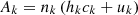$$A_k=n_k\left(h_k{c}_k+u_k\right)$$(2)

The angles u_k are related to the surface powers P_k and curvatures c_k by the paraxial refraction formula$$n_{k+1}{u}_{k+1}=n_k{u}_k-h_k{P}_k=n_k{u}_k-h_k{c}_k\left(n_{k+1}-n_k\right).$$(3)

If surface k is aspheric and is described as a spherical surface plus a polynomial, then G_k is the fourth-order radial coefficient appearing in the polynomial.

In the above formulas the angle u_k and the refractive index n_k are those before refraction at surface k, whereas the index k+1 denotes the corresponding values after refraction (see Fig. 1). For each lens m, with m = 1…L, the first surface has index k = 2m−1 and the second surface has k = 2m. Outside of the lenses, the refractive indices are $n_{2m-1}=1$, and inside the lenses we have $n_{2m}=n$. The marginal ray angles before the first and after the last lens of the thin lens group will be denoted by $u_1=\alpha$ and $u_{2L+1}=\beta$ respectively.

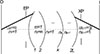Figure 1 The paraxially traced marginal ray (thick line) has before the first surface of the group of L lenses the angle $u_1=\alpha$with the optical axis and after the last surface the angle $u_{2L+1}=\beta$. The refractive index before surface k is $n_k$, after the surface it is $n_{k+1}$.The surface numbering for the marginal ray angles $u_k$is the same. Inside each lens (i.e. for even k values) the refractive index is n, as shown here for the first lens (m=1) with surfaces 1 and 2. Outside the lenses we have $n_1=n_3=...=n_{2L+1}=1$. In this figure, the L lenses of interest form the entire optical system, but the same notation is used when these lenses are part of a larger system. The planes of the object, image, entrance pupil and exit pupil are denoted by O, I, EP and XP respectively. In the thin-lens approximation, all axial distances between surfaces 1 and 2L will be set equal to zero in the aberration formulas.

2.2 Derivation of the simple spherical aberration expression

Readers primarily interested in the results may skip directly to Section 2.3.

To obtain S expressed entirely in terms of the angles u_k, we write A_k as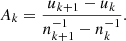$$A_k=\frac{u_{k+1}-u_k}{n_{k+1}^{-1}-n_k^{-1}}.$$(4)

If equation (3) is used to eliminate $u_{k+1}$ in equation (4), then after simple algebra the refraction invariant A_k becomes the one given by the more familiar equation (2).

To shorten the formulas, consider first only spherical surfaces, i.e. we have G_k = 0 for all surfaces (the G_k terms will be included later). Because in the thin-lens approximation all distances between the surfaces shown in Figure 1 are considered to be zero, the height of the marginal ray does not change inside this group and we have 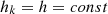$h_k=h=\mathrm{const}$ for all k = 1…2L. For thin lenses in contact, the contributions S_k for odd and even surface numbers result from equations (1) and (4) after simple algebra as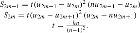$$\begin{array}{c}{S}_{2m-1}=t{\left(u_{2m-1}-u_{2m}\right)}^2\left(n{u}_{2m-1}-u_{2m}\right)\\ S_{2m}=t{\left(u_{2m}-u_{2m+1}\right)}^2\left(u_{2m}-n{u}_{2m+1}\right)\\ t=\frac{\mathrm{hn}}{{\left(n-1\right)}^2}.\end{array}$$(5)

These two surface contributions can be combined as$$S_k={\left(-1\right)}^{k-1}t{\left({\tilde{u}}_k-u_{2m}\right)}^2\left(n{\tilde{u}}_k-u_{2m}\right),$$(6)

where for odd-index angles we introduce the notation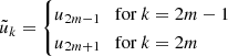$${\tilde{u}}_k=\{\begin{array}{c}{u}_{2m-1}\hspace{1em} \mathrm{for} k=2m-1\\ u_{2m+1}\hspace{1em} \mathrm{for} k = 2m\end{array}$$(7)

To derive the new spherical aberration formula for thin lenses in contact, we start by observing that the surface contributions S_k in equation (6) contain an almost perfect cube of the angle difference ${\tilde{u}}_k-u_{2m}$, the obstacle being the refractive index appearing in the last bracket. As a first step, we show below that the surface contributions can be written as a perfect cube plus correction terms that give the departure from the cube, such that most of the correction terms cancel each other out during summation over surfaces. To facilitate the construction of these expressions, we also introduce temporary variables μ_k, that in air are equal to the corresponding angle u_k, and inside the lens differ from the angle by a factor q that needs to be determined,$${\mu }_{2m-1}=u_{2m-1}, {\mu }_{2m}=q{u}_{2m}.$$(8)

We see from equations (6) and (7) that if we expand S_k we obtain four terms of total power 3 in the angles u, e.g. for the first surface the result will contain terms corresponding to 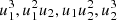$u_1^3,u_1^2{u}_2,u_1{u}_2^2,u_2^3$. In the new variables given by equation (8) S_k will also contain four terms, with coefficients $c_{S1},c_{S2},c_{S3},c_{S4}$ that need to be determined,$$S_k={\left(-1\right)}^{k-1}\left[c_{S1}{\left({\mu }_{2m}-{\tilde{\mu }}_k\right)}^3+c_{S2}{\tilde{\mu }}_k^3+c_{S3}{\mu }_{2m}^3+c_{S4}{\tilde{\mu }}_k^2{\mu }_{2m}\right],$$(9)

where for odd indices ${\tilde{\mu }}_k$is defined in the same way as ${\tilde{u}}_k$in equation (7). Because the goal of this approach is to construct an expression containing a perfect cube, we use the perfect cube in equation (9) instead of the term ${\mu }_{2m}^2{\tilde{\mu }}_k$. Consider first the odd surfaces, for which we have ${\left(-1\right)}^{2m-2}=1$. By substituting equations (8) and (7) into equation (9) we obtain an expression for $S_{2m-1}$ in terms of the angles u that must be equal to that of $S_{2m-1}$ in the first of equation (5). By subtracting the two equivalent expressions for $S_{2m-1}$, and by using e.g. m = 1, we obtain after elementary algebra the zero polynomial$$0=t{\left(u_1-u_2\right)}^2\left(n{u}_1-u_2\right)-c_{S1}{\left(q{u}_2-u_1\right)}^3-c_{S2}{u}_1^3-c_{S3}{q}^3{u}_2^3-c_{S4}q{u}_2{u}_1^2=u_1^3\left(c_{S1}-c_{S2}+\mathrm{tn}\right)-u_2^3\left(q^3\left(c_{S1}+c_{S3}\right)+t\right)-u_2{u}_1^2\left(q\left(3c_{S1}+c_{S4}\right)+\left(2n+1\right)t\right)+u_2^2{u}_1\left(3c_{S1}{q}^2+\left(n+2\right)t\right)$$(10)

By annulling the coefficients of the four terms of total power 3 in the angles u we obtain four equations with five unknowns. We can freely choose one of these unknowns, which are the four coefficients c_S and q. To simplify the construction of the new expression in equation (9), we choose $c_{S4}=0$. After substituting for t the value given in equation (5) we obtain the system of equations 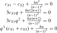$$\begin{array}{c}{c}_{S1}-c_{S2}+\frac{h{n}^2}{{\left(n-1\right)}^2}=0\\ 3c_{S1}q+\frac{\mathrm{hn}\left(2n+1\right)}{{\left(n-1\right)}^2}=0\\ \begin{array}{c}3c_{S1}{q}^2+\frac{\mathrm{hn}\left(n+2\right)}{{\left(n-1\right)}^2}=0\\ q^3\left(c_{S1}+c_{S3}\right)+\frac{\mathrm{hn}}{{\left(n-1\right)}^2}=0\end{array}\end{array}$$(11)

The 2nd and 3rd equation give, after moving one term to the other side, followed by division$$q=\frac{n+2}{2n+1}.$$(12)

Note that if we set n = 1 in equation (12) we obtain q = 1. Because we have $n_{2m-1}=1$, and $n_{2m}=n$, equation (8) can also be written as ${\mu }_k=\left(n_k+2\right)u_k/\left(2n_k+1\right)$.

From the 2nd and first equation in equation (11) we obtain immediately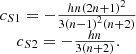$$\begin{array}{c}{c}_{S1}=-\frac{\mathrm{hn}{\left(2n+1\right)}^2}{3{\left(n-1\right)}^2\left(n+2\right)}\\ c_{S2}=-\frac{\mathrm{hn}}{3\left(n+2\right)}.\end{array}$$(13)

The coefficient $c_{S3}$ results from the last of equation (11) but, as will be seen below, it is not important.

Because for $S_{2m}$ we have in equation (9) the factor 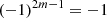${\left(-1\right)}^{2m-1}=-1$, the coefficients $c_{S1},c_{S2},c_{S3}$appear with a sign opposite to that in $S_{2m-1}$. Using equations (7) and (9) we can then write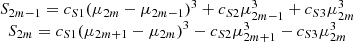$$\begin{array}{c}{S}_{2m-1}=c_{S1}{\left({\mu }_{2m}-{\mu }_{2m-1}\right)}^3+c_{S2}{\mu }_{2m-1}^3+c_{S3}{\mu }_{2m}^3\\ S_{2m}=c_{S1}{\left({\mu }_{2m+1}-{\mu }_{2m}\right)}^3-c_{S2}{\mu }_{2m+1}^3-c_{S3}{\mu }_{2m}^3\end{array}$$(14)

Note that in the first term of $S_{2m}$ we have changed the order of ${\mu }_{2m+1}$ and ${\mu }_{2m}$ compared to equation (9), therefore $c_{S1}$appears here with the plus sign.

We now replace the temporary variables ${\mu }_k$by the new variables $z_k=({\mu }_{k+1}-{\mu }_k)/(\beta -\alpha )$. The total spherical aberration S is then obtained in terms of the new variables $z_k$ by summing up the odd and even surface contributions in equation (14) over all lenses, with m = 1…L. Note that in this sum all terms with coefficients $c_{S3}$cancel each other out, as well as the terms with coefficients $c_{S2}$, excepting those with ${\mu }_1^3=u_1^3={\alpha }^3,$ and ${\mu }_{2L+1}^3=u_{2L+1}^3={\beta }^3$.

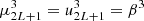2.3 The simple spherical aberration expression

By using equations (8) and (12) the new variables can be rewritten as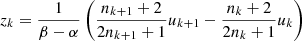$$z_k=\frac{1}{\beta -\alpha }\left(\frac{n_{k+1}+2}{2n_{k+1}+1}{u}_{k+1}-\frac{n_k+2}{2n_k+1}{u}_k\right)$$(15)

and, in the absence of aspheres, spherical aberration becomes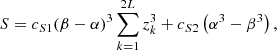$$S=c_{S1}(\beta -\alpha {)}^3\sum _{k=1}^{2L}\mathrm{}{z}_k^3+c_{S2}\left({\alpha }^3-{\beta }^3\right),$$(16)

where $c_{S1}$and $c_{S2}$are given by equation (13).

The marginal ray angles α and β, before and after the thin-lens group, are related to the total power K of the group via$$\beta =\alpha -\mathrm{hK}.$$(17)

Including in equation (16) the aspheric contributions appearing in equation (1) is straightforward because, apart from an alternating sign, the refractive index difference is the same for all surfaces. Using equation (17), we obtain for the spherical aberration of the thin-lens group the final expression$$S=\frac{h^4{K}^{3}n}{3\left(n+2\right)}\left[\frac{{\left(2n+1\right)}^2}{{\left(n-1\right)}^2}\sum _{k=1}^{2L}\mathrm{}{z_k}^3-3{\overline{\alpha }}^2+3\overline{\alpha }-1\right]+8h^4\left(n-1\right)\sum _{k=1}^{2L}\mathrm{}{\left(-1\right)}^{k-1}{G}_k,$$(18)

where we have used the abbreviation$$\overline{\alpha }=\frac{\alpha }{\mathrm{hK}}.$$(19)

If the group of L thin lenses is part of a larger system, then the 3rd-order spherical aberration of the entire system is$$S_{\mathrm{tot}}=S+S^{\mathrm{*}},$$(20)

where S ^* denotes the contribution of the other lenses in the larger system.

3 Quasi-powers and surface powers

The new variables $z_k$defined by equation (15) are essential for simplifying the entire thin-lens formalism and provide a new framework for analysing aberrations. In this section we discuss their properties as well as their relationship with the surface powers and curvatures.

When the angles $u_k$inside the lens group are known, the corresponding $z_k$ values can be determined using equation (15). However, as shown in the Examples section, it is sometimes possible to determine the $z_k$values first. Then, the surface curvatures$c_{k }$result from the $z_k$ values as follows. We find from equations (15) and (17) $${\mu }_{k+1}={\mu }_k+\left(\beta -\alpha \right)z_k={\mu }_k-\mathrm{hK}{z}_k={\mu }_{k-1}-\mathrm{hK}\left(z_k+z_{k-1}\right)=...=\alpha -\mathrm{hK}\sum _{i=1}^k\mathrm{}{z}_i.$$(21)

For k = 2L we expect to have, because of equation (17), 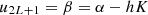$u_{2L+1}=\beta =\alpha -\mathrm{hK}$. The denominator in equation (15) was therefore chosen such that the sum of all z-variables is normalized to unity,$$\sum _{k=1}^{2L}\mathrm{}{z}_k=1.$$(22)

The surface powers result from equations (3) and (8):$$\begin{array}{c}{P}_k=(n_k{u}_k-n_{k+1}{u}_{k+1})/h\\ P_{2m}=\left(\frac{n{\mu }_{2m}}{q}-{\mu }_{2m+1}\right)/h=\left(\frac{n{\mu }_{2m}}{q}-{\mu }_{2m}+\mathrm{hK}{z}_{2m}\right)/h=K{z}_{2m}+\left(\frac{n}{q}-1\right){\mu }_{2m}/h\\ P_{2m-1}=\left({\mu }_{2m-1}-n{\mu }_{2m}/q\right)/h=\left({\mu }_{2m}+\mathrm{hK}{z}_{2m-1}-n{\mu }_{2m}/q\right)/h=K{z}_{2m-1}-\left(n/q-1\right){\mu }_{2m}/h\end{array}.$$(23)

equation (12) gives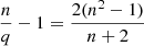$$\frac{n}{q}-1=\frac{2(n^2-1)}{n+2}$$(24)

and from equations (21) and (19) we obtain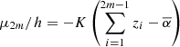$${\mu }_{2m}/h=-K\left(\sum _{i=1}^{2m-1}\mathrm{}{z}_i-\overline{\alpha }\right)$$(25)

The surface powers are then$$\begin{array}{c}{P}_{2m-1}=K\left[z_{2m-1}+\frac{2\left(n^2-1\right)}{\left(n+2\right)}\left(\sum _i^{2m-1}\mathrm{}{z}_i-\overline{\alpha }\right)\right]\\ P_{2m}=K\left[z_{2m} -\frac{2\left(n^2-1\right)}{\left(n+2\right)}\left(\sum _i^{2m-1}\mathrm{}{z}_i-\overline{\alpha }\right)\right]\end{array}$$(26)

and the corresponding surface curvatures result then from equation (3) as$$c_k=P_k/\left(n_{k+1}-n_k\right).$$(27)

It follows from equation (26) that the power of lens m, ${\overline{P}}_m=P_{2m-1}+P_{2m}$ is simply$${\overline{P}}_m=K\left(z_{2m-1}+z_{2m}\right).$$(28)

Note from equations (26) and (28) that, for each lens surface, $z_k$ has a term proportional to the surface power, plus a correction term that is exactly compensated by a correction term of equal magnitude and opposite sign coming from the other surface of the same lens. The power of each lens is then proportional to the sum of the z-values of its two surfaces. Because they can be viewed intuitively as power-like quantities, we refer to the variables $z_k$as “quasi-powers”.

When the group of thin lenses forms the entire system, the position of the object s_o and that of the image s_i with respect to the lens group and the transverse magnification M_T are determined by the angles $u_1=\alpha$ and $u_{2L+1}=\beta$,$$s_o=-h/\alpha , s_i=-h/\beta , M_T=s_i/s_o=\alpha /\beta .$$(29)

Using equations (29), equation (17) becomes after division by h the well-known Lensmaker’s Formula $1/s_i-1/s_o=K$.

4 Other aberrations

4.1 Axial colour, astigmatism and Petzval sum

The simple relation (28) between the power ${\overline{P}}_m$of a lens and the two quasi-powers leads immediately to the expression for the total axial colour of the thin lens group expressed in terms of quasi-powers. As well known, the axial colour contribution of each lens in the group is proportional to its lens power [1]. The total axial colour of the thin lens group is then the sum of the contributions of the individual lenses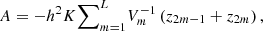$$A=-h^{2}K{\sum }_{m=1}^L\mathrm{}{V}_m^{-1}\left(z_{2m-1}+z_{2m}\right),$$(30)

where V_m is the Abbe number for lens m. When equation (30) is used, the Abbe numbers can be different, but the refractive index n needs to be the same for all lenses in the thin group.

For the thin lens group, several primary aberrations do not depend on the quasi-powers and have well-known expressions [1]. If the aperture stop is placed at the thin lens group, the 3rd-order distortion and lateral colour vanish. The total astigmatism $T_1$and Petzval sum ${T_1}^{\text{'}}$ of the lens group are$$T_1=H^{2}K$$(31)

and$${\mathrm{T\text{'}}}_1=T_1/n,$$(32)

where H is the Lagrange invariant of the entire system.

The last Seidel aberration that remains to be expressed in terms of the quasi-powers is coma. The same approach as for spherical aberration can be used to obtain a simple formula for the coma contribution of thin lenses in contact. The Seidel sum for the 3rd-order coma is [1]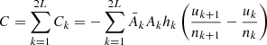$$C=\sum _{k=1}^{2L}\mathrm{}{C}_k=-\sum _{k=1}^{2L}\mathrm{}{\overline{A}}_k{A}_k{h}_k\left(\frac{u_{k+1}}{n_{k+1}}-\frac{u_k}{n_k}\right)$$(33)

When the aperture stop is placed at the group of thin lenses, the chief-ray height at the group is zero. The paraxial refraction invariant ${\overline{A}}_k$for the chief ray (which has a formula similar to equation (2), but using the chief-ray height and angle) is then given by the chief ray angle $\overline{u}$ before and after the group, ${\overline{A}}_k={\overline{u}}_1={\overline{u}}_{2L+1}=\overline{u}$.

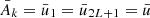4.2 Derivation of the simple coma expression

Readers primarily interested in the results may skip directly to Section 4.3.

For odd and even surfaces we have the surface contributions$$\begin{array}{c}{C}_{2m-1}=t^{\mathrm{\prime }}\left(u_{2m-1}-u_{2m}\right)\left(n{u}_{2m-1}-u_{2m}\right)\\ C_{2m}=t^{\mathrm{\prime }}\left(u_{2m+1}-u_{2m}\right)\left(u_{2m}-n{u}_{2m+1}\right)\\ t\text{'}=\frac{h\overline{u}}{n-1}\end{array}$$(34)

or, using equation (7) $$C_k={\left(-1\right)}^{k-1}{t}^{\mathrm{\prime }}\left({\tilde{u}}_k-u_{2m}\right)\left(n{\tilde{u}}_k-u_{2m}\right).$$(35)

When expanded, the coma surface coefficient contains three quadratic terms in the angles u. We look for new forms of equation (34) as a perfect square plus two correction terms. For odd surfaces we look for a form$$C_{2m-1}=c_{C1}{\left({\mu }_{2m}-{\mu }_{2m-1}\right)}^2+c_{C2}{\mu }_{2m-1}^2+c_{C3}{\mu }_{2m}^2.$$(36)

If in equation (36) we substitute equation (8) and expand the square, the resulting expression must be equal to the expanded form of the first of equation (34). Subtracting these two expressions gives for m = 1 the zero polynomial$$\begin{array}{c}0=t^{\mathrm{\prime }}\left(u_1-u_2\right)\left(n{u}_1-u_2\right)-c_{C1}{\left(q{u}_2-u_1\right)}^2-c_{C2}{u}_1^2-c_{C3}{q}^2{u}_2^2\\ =u_2^2\left(-c_{C1}{q}^2-c_{C3}{q}^2+t\mathrm{\prime }\right)-\left(u_1^2\left(c_{C1}+c_{C2}-\mathrm{nt}\mathrm{\prime }\right)\right)+u_2{u}_1\left(2c_{C1}q-\left(n+1\right)t\mathrm{\prime }\right)\end{array}.$$(37)

After substituting q and t’ using equations (12) and (34) we obtain by annulling the three coefficients of the quadratic terms the system of equations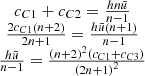$$\begin{array}{c}{c}_{C1}+c_{C2}=\frac{\mathrm{hn}\overline{u}}{n-1}\\ \frac{2c_{C1}\left(n+2\right)}{2n+1}=\frac{h\overline{u}\left(n+1\right)}{n-1}\\ \frac{h\overline{u}}{n-1}=\frac{{\left(n+2\right)}^2\left(c_{C1}+c_{C3}\right)}{{\left(2n+1\right)}^2}\end{array}$$(38)

that gives for $c_{C1}$and $c_{C2}$ ($c_{C3}$will not be needed)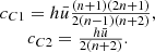$$\begin{array}{c}{c}_{C1}=h\overline{u}\frac{\left(n+1\right)\left(2n+1\right)}{2\left(n-1\right)\left(n+2\right)},\\ c_{C2}=\frac{h\overline{u}}{2\left(n+2\right)}.\end{array}$$(39)

Because of the factor ${\left(-1\right)}^{k-1}$in equation (35), for the even surfaces the three coefficients are exactly the opposite of those in equation (36) and we have$$C_{2m}=-c_{C1}{\left({\mu }_{2m+1}-{\mu }_{2m}\right)}^2-c_{C2}{\mu }_{2m+1}^2-c_{C3}{\mu }_{2m}^2.$$(40)

When we sum up the surface contributions (36) and (40) over all lenses, all $c_{C3}$terms cancel each other out, as well as the $c_{C2 }$terms, excepting those with ${\mu }_1^2=u_1^2={\alpha }^2$, and ${\mu }_{2L+1}^2=u_{2L+1}^2={\beta }^2$.

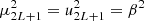4.3 Polynomial pattern

With the new variables defined by equation (15), the quadratic terms appear in the coma expression C with alternating signs,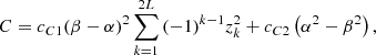$$C=c_{C1}(\beta -\alpha {)}^2\sum _{k=1}^{2L}\mathrm{}{\left(-1\right)}^{k-1}{z}_k^2+c_{C2}\left({\alpha }^2-{\beta }^2\right),$$(41)

where $c_{C1}$and $c_{C2}$are given by equation (39). Alternatively, the coma contribution of the thin lens group, with the stop at the lens group, can be written as$$C=\frac{-\overline{u}{h}^3{K}^2}{2\left(n+2\right)}\left[\frac{\left(n+1\right)\left(2n+1\right)}{n-1}\sum _{k=1}^{2L}\mathrm{}{\left(-1\right)}^k{z_k}^2-2\overline{\alpha }+1\right].$$(42)For an arbitrary stop position, the contribution of the thin lens group to the primary aberrations can be computed by using the well-known stop-shift formulas [1, 2].

Note that, when all surfaces are spherical, all Seidel (monochromatic) aberration formulas have the same structure$$T_j=a_j(\beta -\alpha {)}^j\left({\sum _{k=1}^{2L}\mathrm{}}_{}{\left(-1\right)}^{\left(j+1\right)\left(k-1\right)}{z}_k^j\right)+b_j\left({\alpha }^j-{\beta }^j\right).$$(43)

The exponent of −1 was chosen such that for odd indices j all terms $z_k^j$have the same sign for all values of k, and that for even j the signs of $z_k^j$are alternating. For spherical aberration and coma we have j = 3 and j = 2, respectively, with $T_3=S$given by equation (16) and $T_2=C$given by equation (41), and the coefficients are $a_3=c_{S1},b_3=c_{S2},a_2=c_{C1},b_2=c_{C2}$. The aberrations that have simple expressions also fit into this pattern. For astigmatism and Petzval sum (Eqs. (31) and (32)) we have j = 1. The sum in equation (43) is then 1 because it becomes the constraint (22), therefore both aberrations are constant. According to equation (17), for j = 1 both factors $(\beta -\alpha {)}^j$and ${\alpha }^j-{\beta }^j$ are proportional to the power K, a property that is in agreement with equation (31). The distortion $T_0$ is zero as expected, because for j = 0 the sum with alternating terms in equation (43) is $L-L=0$ and we have ${\alpha }^0-{\beta }^0=1-1=0$.

5 Examples

The thin-lens formulas for primary aberrations derived in this paper have been verified using the lens design programs CODE V and Zemax OpticStudio. For lens systems where distances between surfaces have been set to zero, the quasi-powers are computed using paraxial ray-tracing data and equation (15). Then, as shown in the supplementary data, implementing the new aberration formulas in the macro languages leads to numerical values that are identical with the corresponding coefficients listed by these programs (see the link in the Data availability statement).

5.1 Equal quasi-powers

In the examples below we consider only systems having spherical surfaces. We first focus on the spherical aberration S. We denote the sum of cubes that appears in equations (16) and (18) by $s=\sum _{k=1}^{2L}\mathrm{}{z_k}^3$. If for a system consisting of L lenses the quasi-powers $z_k$are considered to be variables that satisfy the constraint (22), then it can be seen that, because of the perfect symmetry, a system having equal quasi-powers, i.e.$$z_k=1/\left(2L\right),$$(44)

for all k-values, must be an extremum of s. By slightly perturbing this system by a small quantity ε, $z_1=1/\left(2L\right)+\epsilon$ and (to satisfy the constraint) $z_2=1/2L-\epsilon , z_k=1/2L \mathrm{for} k>2$, we obtain $s\left(\epsilon \right)=1/\left(4L^2\right)+3{\epsilon }^2/L$ which is always larger than$$s_{\min }=\frac{1}{\left(4L^2\right)}.$$(45)

Several known results can be easily derived by starting from systems with equal quasi-powers, that are minima of s, with the minimum value $s=s_{\min }$.

For L = 1, we recover familiar results of traditional thin-lens theory. The system with $z_1=z_2=1/2$ corresponds then to the well-known singlet with optimal bending that has minimal spherical aberration. Traditional thin-lens theory uses the magnification variable 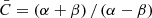$\overline{C}=\left(\alpha +\beta \right)/\left(\alpha -\beta \right)$. Inserting in equation (18) $s_{\min }=1/4$ and $\overline{\alpha }=(1+\overline{C})/2$ leads to the well-known minimal spherical aberration formula [1]$$S_{\min }=\frac{1}{4}{h}^4{K}^{3}n\left(\frac{n}{{\left(n-1\right)}^2}-\frac{{\overline{C}}^2}{n+2}\right).$$(46)

For larger L, an interesting result that has a rather complex derivation in the literature follows easily from the present model. Fulcher has shown that 3rd-order spherical aberration can be corrected with thin lenses having the same power, but different bendings. In his telescope objective, four lenses with a refractive index close to n = 1.5 are used to achieve this goal [3]. For L=4 we have for all k $z_k=1/8$ and $s_{\min }=1/64$. With $\overline{\alpha }=0$(object at infinity) equation (18) leads to$$S_{\min }=-\frac{h^4{K}^{3}n\left(2n-3\right)\left(10n-7\right)}{64{\left(n-1\right)}^2\left(n+2\right)}.$$(47)

Spherical aberration vanishes for n = 1.5 because of the first parenthesis in the numerator. It follows from equation (28) that all four lens powers are equal, ${\overline{P}}_m=K/4$, despite of the fact that the four lenses have different curvatures (the surface powers resulting from equation (26) are the same as those listed in Table 1 of Ref. [3]). As shown by Shafer, Fulcher systems are good starting points for further design and lead to relaxed designs that have an axial imaging of excellent quality even at large apertures [4]. For L = 2, converting the four equal quasi-powers in equation (44) into curvatures using equations (26) and (27) leads to a doublet configuration that is also given as a typical example of a relaxed design (see Fig. 1 of Ref. [4]). Figure 2 shows a Fulcher quartet appearing as a lens group in a lithographic objective having only spherical surfaces and a numerical aperture of 0.56. This system is closely related to a system in [5, 6]. The similarity with the lens shapes in the blue box supports the interpretation of the lenses in the red box as essentially a Fulcher group.

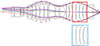Figure 2 Red box: Fulcher group in an optimized design in which all lenses have the same material. Blue box: the shapes of the same four lenses resulting from the present thin-lens model using $z_k=1/8$ and the marginal ray angles α and β before and after the four-lens group, extracted from the optimized design. In the drawing, the lens thicknesses, which are assumed to be zero in the calculations, are kept the same as in the red box.

5.2 Permutation symmetry for spherical aberration

In many imaging systems, including the one shown in Figure 2, we encounter groups of lenses having reasonably small thicknesses and air spaces between them. Simplified models, including the thin-lens approximation used here, rarely yield accurate quantitative results, but the deliberate neglect of distracting complexities can reveal qualitative properties that are otherwise obscured. The principal motivation behind deriving the thin-lens formulas was to provide a simplified framework for gaining insight into the properties of the lens design landscape. Because of the extensive derivations involved, detailed examples will be presented in a separate paper. Here we show an example that helps answering a fundamental question in optical system optimization: why are there so many local minima in the design landscape?

The existence of certain local minima in the optimization landscape can already be explained using 3^rd-order aberrations. If the surrounding landscape is not flat, higher-order aberrations only determine how deep these minima are. In an optimization landscape with specifications that make spherical aberration the most significant aberration, consider for simplicity a rough approximation of the error function, E = S_tot ² . Because in S given by equation (18) the quasi-powers appear in the sum of cubes s, the mathematical property of commutativity leads to permutation symmetry: if a certain set of variables $z_k$corresponds to a local minimum, then any permutation of these variables will have the same values of s, S, S_tot (given by equation (20)) and E. Any such permutation will then correspond to a different minimum, a property that increases the number of existing minima in the landscape significantly. This permutation symmetry was not visible in earlier formalisms, because of the sequential character of ray propagation (rays pass first through surface 1, then through surface 2 etc.). However, the quasi-power formalism reveals this symmetry because the sequential character of ray propagation is now absorbed in equation (26) and is therefore separated from the more important aberration properties resulting from equation (18), or, more generally, from equation (43).

Figure 3 shows an example of the effect of the permutation symmetry in S on the number of local minima. As shown previously [7], local minima in the optimization landscape surrounding the system in Figure 2 generally have localized changes in the corresponding system drawings. The red boxes in Figure 3 contain local minima for which the most significant changes occur within the group of four lenses considered in Figure 2. These systems have been obtained with CODE V, with lens curvatures as optimization variables, and distortion control added to the default error function. For this study, telecentricity was not controlled and edge thickness control inside this lens group was disabled.

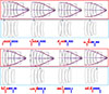Figure 3 Eight local minima in the vicinity of the system in Figure 2 are shown in the red boxes. Only the last six lenses are shown, which include the four lenses of interest. The lenses with the most significant change compared to Figure 2 are marked with an arrow. For the four lenses of interest the blue bar charts show the z-values that result from theory, one negative z-value and seven equal positive z-values. When these z-values are translated into surface curvatures, the lenses in the blue boxes are obtained. For comparison, the red bar charts show the z-values obtained from data extracted from the optimized systems.

In Figure 3 we consider the same group of four lenses as in Figure 2. For the upper left local minimum, the model assigns one negative and seven identical positive z-values to the four lenses, as illustrated by the corresponding blue bar chart. (Theory – partly already developed in [8] and to be presented in detail in a separate work – predicts the existence of such minima, characterized by one negative and seven equal positive z-values, in the vicinity of a Fulcher-like group having eight equal z-values.) The permutation symmetry in S then implies the existence of seven additional local minima, in which the negative z-value of the first minimum appears at each of the other positions within the group. The permuted z-values are shown by the blue bar charts. The lenses enclosed by blue boxes are obtained by translating each of the eight permuted sets of z-values into surface curvatures using equations (26) and (27).

The systems in red boxes are candidates for the predicted local minima in the optimization landscape. The red bar charts show for these systems the z-values obtained using equation (15) and marginal-ray data from the optimized systems. Some discrepancy between the red and blue bars is expected, because the approximate error function E neglects many aberrations and because the model assumes zero-thickness lenses, whereas the optimized systems contain lenses of finite thickness. (Also, the red bars show seemingly larger discrepancies because they show relative rather than absolute differences, and because the z-values for the four surfaces of interest are significantly smaller than those of more strongly curved surfaces elsewhere in the system.) However, for the systems in red boxes the shapes of the four lenses of interest agree reasonably well with the corresponding lenses in blue boxes. This agreement supports the interpretation of these systems as the eight minima resulting from permutation symmetry.

5.3 Aplanatic correction

In the special case of Fulcher-like thin-lens systems it can be easily seen that the 3rd-order coma formula (equation (42)) is also consistent with traditional aberration theory. For equal quasi-powers (as in equation (44)) the alternating sum of squares in the coma formula vanishes. Coma itself then vanishes for $\overline{\alpha }=1/2$, which corresponds to the case of equal conjugates (i.e. transverse magnification $M_T=-1$ in equation (29)). However, if the stop is at the lens, the system is symmetric with respect to the stop, and the zero-coma value can also be derived from the traditional symmetry principle [9].

While in the traditional approach the total values of the Seidel aberrations result only from sums over surfaces, in the present approach the corresponding totals in e.g. equation (43) include constant terms in addition to the sums of quasi-power terms over the surfaces. 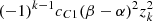In equations (16) for spherical aberration and (41) for coma we can consider the terms $c_{S1}(\beta -\alpha {)}^3{z}_k^3$and ${\left(-1\right)}^{k-1}{c}_{C1}(\beta -\alpha {)}^2{z}_k^2$to be the “quasi-power surface contributions”. The constant terms are then $c_{S2}\left({\alpha }^3-{\beta }^3\right)$ and $c_{C2}\left({\alpha }^2-{\beta }^2\right)$, respectively. The example below shows that, numerically, the quasi-power surface contributions can differ significantly from the corresponding traditional ones. Using the Fulcher approach to annul spherical aberration and symmetry to annul coma, the thin triplet with equal conjugates shown in Figure 4 can achieve 3rd-order aplanatic correction in the infrared region. 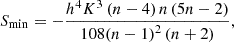For spherical aberration, the equivalent of equation (47) for L = 3 and $\overline{\alpha }=1/2$ (which corresponds to $M_T=-1$) is$$S_{\min }=-\frac{h^4{K}^3\left(n-4\right)n\left(5n-2\right)}{108{\left(n-1\right)}^2\left(n+2\right)},$$(48)

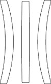Figure 4 Aplanatic thin triplet for the infrared region (n = 4), with an effective focal length of 1, and transverse magnification $M_T=-1$. The zero distances between surfaces are drawn for clarity as finite. The stop is at the thin lens. All six quasi-powers are equal to 1/6. Despite of the different bendings, the three spherical lenses have the same lens power 1/3 (see Eq. (28)).

which becomes zero for n = 4 (germanium in infrared).

For the triplet shown in Figure 4 the quasi-powers z_k and the corresponding surface radii $R_k=\frac{1}{c_k}$resulting from equations (26) and (27) are listed in Table 1, together with aberration coefficients computed using an entrance pupil diameter of 1, and a field angle of 10 degrees. We then have $\alpha =1/4,\beta =-1/4$. While for spherical aberration the traditional surface contributions vary significantly (note for instance that surfaces 1 and 6 are aplanatic), all quasi-power surface contributions are identical (because the z-values are identical, their cubes are also identical). The zero total spherical aberration is achieved due to the constant term, which has the opposite sign and six times the magnitude of the surface contributions. For coma, all quasi-power surface contributions have the same magnitude, but their total vanishes because of their alternating signs.

In the system shown in Figure 4 three lenses have been used to correct 3^rd-order spherical aberration and coma. It is well-known that in fact only two thin lenses are sufficient for annulling, not only these two aberrations, but axial colour as well, while keeping the desired value of the focal length [2]. (Four solutions can be found, and it will be shown in a future publication that the quasi-power approach can explain the reason why the number of possible solutions is precisely four.) However, the approach used above, called by Shafer the “relaxation design method” [4], achieves, as in the Fulcher case, more than just annulling spherical aberration for appropriate values of α, β, and n. The fact that spherical aberration given by equation (48) is also an extremum with respect to small changes of quasi-power leads to a flat design landscape around the solution in Figure 4. Pioneered by Glatzel, the “relaxation design method” is especially useful for systems having a high numerical aperture, due to better tolerances and reduced high-order aberrations, but often at the cost of an increased element count [4]. It is therefore unsurprising that Fulcher-like groups are often encountered as building blocks in lithographic objectives like the one shown in Figure 2. (There, a 2^nd Fulcher-like building block can be found in the first wide group of lenses.)

Conclusion

This paper introduces a novel framework for analysing the aberrations of thin lenses, based on the concept of surface quasi-power. The equation (43) shows that in this framework all Seidel aberrations follow the same remarkably simple polynomial pattern. Apart from a constant term, the aberrations become essentially sums over all surfaces of powers of the new variables. However, even in the zero-thickness limit the contribution of a surface in the present formalism is not the same as the corresponding classical Seidel surface contribution.

In the examples, several classical lens design results follow naturally from the new formalism, in some cases with a simpler derivation than the one found in the existing literature. Optimal singlet bending, relaxed doublets and Fulcher configurations can all be understood as a direct consequence of quasi-power equality. Although the thin-lens approximation employed here is not intended to yield quantitatively accurate predictions, it can serve as a qualitative model that separates the essential properties of primary aberrations from secondary factors.

When expressed in terms of quasi-powers, spherical aberration becomes independent of the internal surface ordering. This property explains the occurrence in the optimization landscape of large families of local minima through permutation symmetry – a property that is already present at the level of third-order theory. Extensions of this work, including more detailed analyses of the design landscape and higher-order effects, will be addressed in a future publication.

Funding

This research was funded by TU Delft.

Conflicts of interest

The author has nothing to disclose.

Data availability statement

Test lenses, a CODE V and a Zemax macro, the corresponding outputs and the Zemax lens for the system in Figure 4 are available at https://doi.org/10.4121/ecc198ad-889a-4ea6-aebb-302303f4e999.

Acknowledgments

The author gratefully acknowledges the use of academic licenses for CODE V and Zemax OpticStudio. The author would also like to thank Kumar Rishav for his assistance with the data presented in Figure 3.

References

All Tables

All Figures

Figure 1 The paraxially traced marginal ray (thick line) has before the first surface of the group of L lenses the angle $u_1=\alpha$with the optical axis and after the last surface the angle $u_{2L+1}=\beta$. The refractive index before surface k is $n_k$, after the surface it is $n_{k+1}$.The surface numbering for the marginal ray angles $u_k$is the same. Inside each lens (i.e. for even k values) the refractive index is n, as shown here for the first lens (m=1) with surfaces 1 and 2. Outside the lenses we have $n_1=n_3=...=n_{2L+1}=1$. In this figure, the L lenses of interest form the entire optical system, but the same notation is used when these lenses are part of a larger system. The planes of the object, image, entrance pupil and exit pupil are denoted by O, I, EP and XP respectively. In the thin-lens approximation, all axial distances between surfaces 1 and 2L will be set equal to zero in the aberration formulas.

In the text

Figure 2 Red box: Fulcher group in an optimized design in which all lenses have the same material. Blue box: the shapes of the same four lenses resulting from the present thin-lens model using $z_k=1/8$ and the marginal ray angles α and β before and after the four-lens group, extracted from the optimized design. In the drawing, the lens thicknesses, which are assumed to be zero in the calculations, are kept the same as in the red box.

In the text

Figure 3 Eight local minima in the vicinity of the system in Figure 2 are shown in the red boxes. Only the last six lenses are shown, which include the four lenses of interest. The lenses with the most significant change compared to Figure 2 are marked with an arrow. For the four lenses of interest the blue bar charts show the z-values that result from theory, one negative z-value and seven equal positive z-values. When these z-values are translated into surface curvatures, the lenses in the blue boxes are obtained. For comparison, the red bar charts show the z-values obtained from data extracted from the optimized systems.

In the text

	Figure 4 Aplanatic thin triplet for the infrared region (n = 4), with an effective focal length of 1, and transverse magnification $M_T=-1$. The zero distances between surfaces are drawn for clarity as finite. The stop is at the thin lens. All six quasi-powers are equal to 1/6. Despite of the different bendings, the three spherical lenses have the same lens power 1/3 (see Eq. (28)).
In the text

References

- Welford WT, Aberrations of Optical Systems (Adam Hilger, Bristol, 1986). [Google Scholar]
- Sasian J, Introduction to Aberrations in Optical Imaging Systems (Cambridge University Press, Cambridge, 2013). [Google Scholar]
- Fulcher GS, Telescope objective without spherical aberration for large apertures, consisting of four crown glass lenses, J. Opt. Soc. Am. 37, 47 (1947). https://doi.org/10.1364/JOSA.37.000047. [Google Scholar]
- Shafer D, Optical design and the relaxation response, Proc. SPIE 0766, 2 (1987). https://doi.org/10.1117/12.940196. [Google Scholar]
- Sasaya T et al., Projection optical system and projection exposure apparatus, U.S. Patent 5,805,344 (1998). [Google Scholar]
- Caldwell JB, All-fused silica 248-nm lithographic projection lens, Opt. Photon. News 9, 40 (1998). https://doi.org/10.1364/OPN.9.11.000040. [Google Scholar]
- Marinescu O, Bociort F, Saddle-point construction in the design of lithographic objectives, part 1: method, Opt. Eng. 47, 093002 (2008). https://doi.org/10.1117/1.2981512. [Google Scholar]
- Bociort F, Why are there so many system shapes in lens design? Proc. SPIE 7849, 78490D (2010). https://doi.org/10.1117/12.873880. [Google Scholar]
- Gross H et al., Handbook of Optical Systems, Vol.3 (Wiley-VCH, Weinheim, 2007). [Google Scholar]
All Tables
The quasi-power surface contributions for spherical aberration (QPS) and coma (QPC) differ significantly from the corresponding traditional surface contributions for spherical aberration (Trad. S) and coma (Trad. C). The constant terms (Const.), which are absent (–) in the traditional approach, are also listed in the QPS and QPC columns. The values in the columns Trad. S and Trad. C are identical with the corresponding Seidel coefficients SPHA S1 and COMA S2 listed by Zemax.