| Issue |
J. Eur. Opt. Society-Rapid Publ.
Volume 21, Number 1, 2025
EOSAM 2024
|
|
|---|---|---|
| Article Number | 27 | |
| Number of page(s) | 19 | |
| DOI | https://doi.org/10.1051/jeos/2025017 | |
| Published online | 27 June 2025 | |
Research Article
An integrated exposure and measurement tool for 5-DOF direct laser writing based on chromatic differential confocal sensing
Technische Universität Ilmenau, Department of Mechanical Engineering, Institute of Process Measurement and Sensor Technology, Gustav-Kirchhoff-Straße 1, 98693 Ilmenau, Germany
* Corresponding author: This email address is being protected from spambots. You need JavaScript enabled to view it.
Received:
31
January
2025
Accepted:
1
April
2025
Abstract
Accurate and uniform fabrication of microstructures on highly curved substrates requires exposure with the waist of a focused laser beam at every point. In order to realize this, the exposure beam must be held perpendicular and focused onto the local substrate. Here we present an optical tool for our developed 5-axis nano-positioning and nano-measurement machine based on the chromatic differential confocal microscope. Thereby, we introduce the optical design methodology to realize high axial sensitivity from differential optical feedback via axial chromatic aberration. Additionally, the deflection angle is measured via a camera sensor to provide angular feedback. Overall, our probe attains a nanometer axial sensitivity and arc-minute angular sensitivity in a confined space of 50 × 80 × 36 mm3.
Key words: Differential confocal microscopy / Chromatic optical design / Nano-positioning
© The Author(s), published by EDP Sciences, 2025
 This is an Open Access article distributed under the terms of the Creative Commons Attribution License (https://creativecommons.org/licenses/by/4.0), which permits unrestricted use, distribution, and reproduction in any medium, provided the original work is properly cited.
1 Introduction
Flexible prototyping of microstructures via direct laser writing (DLW) or laserablation recently enabled a whole new field for the creation of micro-optics [1, 2], micro-fluidics [3, 4], MEMS [5, 6] and metamaterials [7, 8]. Thereby, a single laser spot exposes or ablates a small volume of photoresist on a substrate. Using multiphoton absorption in DLW, this even allowed for the creation of extended complex three-dimensional structures [9, 10].
The fabrication on, and modification of, highly curved substrates such as lenses, mirrors or free-form substrates, however, remains an open challenge. The accurate structuring of such substrates could enhance the manufacturing of hybrid diffractive-refractive optical elements, highly integrated systems such as wearables [11, 12] or new approaches for classic [13], optical [14] and organic circuit design [15].
In order to achieve highest accuracy at the current point of structuring on the substrate (POS), the optical tool needs to follow local surface slope as indicated by the tilted objective in Figure 1. A current project at our institute is the metrological 5-axis nano-positioning and nano-measuring machine (NPMM-5D) [16], also shown in Figure 1, that allows to position and rotate around the POS with nanometer-accuracy by following the extended Abbe-principle [17]. Thereby, all position measurement axes and the tool focus must intersect in the POS as indicated by the dashed lines in Figure 1. For the rotations, the spherical position measurement is realized by encoders in rotational actuators, but expanded by Fabry-Pérot interferometers that observe the eccentricity towards a reference hemispherical mirror. This limits the available space for tool-heads to 50 × 80 × 36 mm3 and therefore requires innovative miniaturized measurement and structuring systems. Such a miniature tool-head has to provide three major functions. At first, the tool-head shall realize a small structuring spot for nano-fabrication. Here we aim for the exposure of photoresist and therefore the employment of a blue diode laser. Second, the tool-head must provide a feedback signal for the three Cartesian nano-positioning axes to keep the substrate surface within the focal spot of said structuring beam. Third, to adjust the tool-heads structuring axis towards the surface slope, angular feedback signals must be generated for the rotational nano-positioning axes. Finally, as a secondary functional requirement, the integration of a wide-field microscope for manual rough positioning would be desirable.
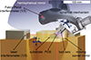 |
Figure 1 CAD model view of the significant parts of the NPMM-5D. |
1.1 Optical feedback systems
As the generation of a diffraction limited structuring laser spot can be realized easily by focusing a collimated beam with a suitable precision asphere. A major challenge in optical design is the integration of an optical surface feedback system that works online. This means that the substrate is assumed to be of unknown shape and cannot be compensated by feed-forwarding its profile to the trajectory planner of the NPMM-5D. Suitable feedback systems therefore must be fast enough for the positioning axes that run at 10 kHz. Optically, such systems must provide a point of measurement that aligns with the POS. It should provide nanometer height resolution to achieve homogeneous exposure. Thereby, the measurement wavelength must be sufficiently far from exposure wavelength to prevent undesired structuring. Furthermore, it must be possible to miniaturize and integrate it within the given space for the tool-head. In agreement with the alignment of the probing point and the POS, a common axis for both systems with a common coupled fiber would be advantageous for easier integration into the small building volume.
Optical surface probing of microscopic specimens is a widely studied field of science. Possible principles can be generally classified into interferometric and non-interferometric systems. A prominent example for the former category is coherence scanning interferometry [18], confocal microscopy is an example for the latter [19]. Both require axial scanning to reconstruct the surface profile and therefore are not suitable for the required online feedback demanded by the in this article discussed application.
A further advanced interferometric technique is Fourier domain optical coherence tomography (FD-OCT). FD-OCT can achieve nanometer axial resolution in a single spectral acquisition cycle [20]. However, complex broadband sources, such as sweeping laser sources, are typically used to realize the necessary spectral resolution, leading to the necessity of tight dispersion control between measurement and reference arm [21]. Furthermore, interferometric systems are sensitive to all vibrations and other parasitic drifts occurring between the reference and measurement arm. Therefore, placement of the reference close to the substrate is often necessary to maintain stability, which leads to a larger beam-path and incompatibility with the exposure beam.
A non-interferometric approach could be the employment of chromatic confocal microscopy (CCM) [22]. Due to axial chromatic aberration in the focusing objective, broadband light is focused onto different axial planes. The substrate’s surface then would cause an axial confocal signal along the spectrum. For well designed chromatic objectives, this spectral axis would be linear towards the depth of the substrate [23]. By using peak fitting and reconstruction algorithms, nanometer axial resolution can be achieved in a single acquisition cycle [24]. Compared to an FD-OCT system, not requiring a reference arm, is expected to provide measurements at comparable axial resolution, but with higher stability. This requires a sufficiently high resolution of the spectral confocal peak, which for typical spectrometers require a broader spectrum. This may lead to longer evaluation times and incompatibility to a common single-mode fiber.
FD-OCT and CCM both require axially distributed probing points to reconstruct the surface position via the knowledge of the whole peak. A less data intensive approach and therefore faster evaluation emerges from the analysis of the axial response signal of a classic confocal microscope. As shown in Figure 2 this ideally resembles a sinc2-peak for Iz [25]. The abscissa of the diagram u is given in normalized axial optical coordinates [26]: (1)
(1)
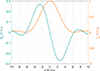 |
Figure 2 Axial confocal response Iz and its sensitivity Sz, alias the differential confocal signal. |
Thereby, λ is the employed effective wavelength and θmax the semi-aperture angle of the objective for NA < 0.5. Iz has a maximum signal response, if the surface of a flat substrate is in the focal plane of the objective at the measurement wavelength. Without any additional information, such a peak signal has two additional drawbacks for online feedback. First, the intensity value is ambiguous. A deviation from the focal plane can not immediately be assorted to a direction for a following correction. Second, looking at the sensitivity Sz of such a peak signal in Figure 2, at the maximum of the peak, the sensitivity is zero. Small deviations might not be detected with noisy systems. Contrary, Sz solves both these issues by its steep slope at the zero-crossing and non-ambiguous range u ⊂ [−2, 2]. Therefore, it would be advantageous to find an optical probe, that can provide a (pseudo-)derivative of the confocal peak signal.
1.2 Chromatic differential confocal microscopy
Systems that can provide such derivative signals towards the surface are called differential optical probes. Famous representatives of these for surface probing are laser focus sensing (LFS) [27] and differential confocal microscopy (DCM) [28]. LFS may be realized with Focault’s knife edge [29], astigmatism [30] or two orthogonal line-gratings [31]. The latter thereby had been miniaturized and widely applied in optical disk drives and has proven useful for nanometer surface probing. However, it is incompatible with the high-integration approach through a single common single-mode fiber (herein after: common fiber).
In DCM the confocal principle is expanded by the arrangement of source- and/or detection-pinholes. Most common is the approach to use two defocused point-detectors. These are symmetrically axially defocused from the focal plane of the detection tube lens [32]. The two acquired signals are then taken into difference Δ and are normalized by their sum Σ to create the so called focus error signal (FES) [33]: (2)
(2)
Early works already managed to achieve nanometer sensitivity [34]. Many works then improved this method regarding robustness [33–36], axial resolution [32, 33], lateral resolution [37, 38], the extension of its non-ambiguous range for direct measurement [39, 40], and parallelization for faster measurements [41]. Further methods to create a DCM developed. The divided aperture method could simplify the detection path by using a single camera that observes light from a partially illuminated objective pupil [42]. While the discussed methods involve static defocus, recently dynamically defocusing to create a differential curve re-emerged [43, 44]. Thereby, the focal plane of the objective has been axially modulated, or the detection plane of the tube lens. This allowed to achieve nanometer axial sensitivity by using a simple confocal beam-path.
However, these methods employing static defocused point detectors or addtitional optical elements require space and different beam-paths of illumination and detection. Therefore, we suggest the rarely employed approach to exploit axial chromatic aberration to create the defocus between two confocal signals [45]. This enables the creation of a differential curve from two wavelengths focused into different focal planes in front of the objective, while using a common fiber for illumination and detection. This target beam-path is sketched in Figure 3. Two confocal peaks will appear at different distance from the objective. This allows for the application of equation (2). Opposite to FD-OCT and CCM, the spectrometer is reduced to two wavelength-specific photodetectors, which enables fast signal processing. A key challenge is to create this axial chromatic aberration for the two long measurement wavelengths, while being achromatic towards the exposure wavelength of the structuring beam.
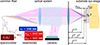 |
Figure 3 Target schematic of the optical tool, integrated with a chromatic differential confocal probe and its required axial chromatic separation of focal planes. Additionally, angular measurements are realized through a camera chip. |
Here we present our approach to design such an optical probe. Section 2 proposes a design procedure for the axial chromatic design. Section 3 briefly integrates an angular measurement beam-path and a possibility for wide-field observation. Furthermore, it introduces the complete realized tool head. Section 4 shows results that characterize the realized measurement systems and demonstrates measurements on a grating and a sphere. Afterwards, Section 5 discusses these measurements and draws connections to the design approach. Finally, the article is concluded in Section 6.
2 Chromatic optical design
As required by the chromatic differential confocal principle [45], the measurement is performed by two wavelengths, λC1 and λC2. Henceforth, their median wavelength may be defined as their effective wavelength λC. The optical design procedure now has to join the exposure tool beam with the wavelength λF and the effective measurement beam as illustrated by Figure 3. All three wavelength are emitted from a common fiber facet. That common fiber shall pose as receiver after reflection on the substrate’s surface, too. The first primary design goal is the achromatism between the focal lengths of the exposure f
F and the effective measurement wavelength f
C: (3)
(3)
The second primary design goal stems from the chromatic differential confocal principle. The axial defocus zD1/2 between the focal planes fC1/2 of the two measurement beams decides for the axial sensitivity, range and signal to noise ratio (SNR) of the resulting differential curve. In normalized axial optical distances this is given as uD,opt = 5.61 as shown in other works [32, 46]. According to equation (1), the relationship between the normalized uD and a real zD is scaled by the employed wavelength and the acting NA. For simplification of the design process, it is suggested, to maximize the zD as the second primary design goal: (4)
(4)
To furthermore maximize design robustness, axial symmetry can be demanded for the respective zD. It is this second primary goal that is unique among the typical design process of chromatic systems. While achromats and apochromats only try to realize demand (I) and similar ([47], p. 313ff), chromatic confocal systems only try maximize demand (II) by their request for large axial chromatic aberration [23, 48, 49].
Other secondary goals shall be the use of off-the-shelf optics, the minimization of optical elements, the minimization of the total length and the minimization of all three lateral spot-sizes for tightly localized exposure and measurement.
To design the required beam-path, the typical design methodology for optical systems is followed [50]. At first, analytical calculations with reduced complexity are desired to find a possibly working start system. In a second major design step, this start system is considered in full complexity and optimized in a commercial ray-tracing software. Here, we in particular focus on the first step and propose a new paraxial design procedure to find the important start system.
2.1 Paraxial chromatic theory
Paraxial theory shall be employed to estimate a start system for the optical beam-path of the chromatic differential confocal probe. Thereby, the space of free design parameters is reduced to the number of lenses, their respective focal length and their chosen lens materials. As shown in Appendix A.1, for an arrangement of k lenses as illustrated in Figure 4, the power of the system from the first to the kth lens can be described recursively as: (5)
(5)
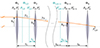 |
Figure 4 Schematic of paraxial ray crossing a system of k thin lenses characterized by their principal planes Pi, |

Thereby, t is the distance from the image-side principal plane of the previous sub-system from the first to the (k − 1)th lens to its (k − 1)th lens: (6)
(6)
For k = 2 follows here the known equation for the power of two lenses Φ1,2 ([47], p. 154). For direct calculation, this recursive equation (5) can also be expressed as a series: (7)
(7)
This series can reproduce the given example in ([47], p. 158) for a system of three lenses. Together with equation (6) it can be used for the convenient estimation of the optical power of larger systems.
To find measures for the axial chromatic aberration, the material properties must be integrated. Widely used are the normalized Abbe number and the partial dispersion. The Abbe number is defined as: (8)where the indices [F, d, C] define the evaluated wavelengths for the design. These may deviate from the original or official definition to meet the given design task. F represents the shortest wavelength of the targeted application spectrum, here the exposure wavelength. d represents a center wavelength of the spectrum. It should correspond with the design wavelength of the respective optical element. C is the longest wavelength of the targeted application spectrum. Here it represents the effective or median measurement wavelength. A higher Abbe number corresponds to lower dispersion. Therefore, it is relevant for achieving goal (I).
The second important normalized material parameter is the partial dispersion. It is defined as: (9)
(9)
The higher ϱ is, the higher the dispersion of the longer wavelength. Therefore, ϱ is important for achieving a high axial chromatic dispersion for goal (II).
First, the achromatism (I) shall be achieved by observation of the change ΔΦ
FC = Φ
F − Φ
C over the spectrum. For a system of k lenses, the achromatic demand must be satisfied by the power difference of the whole system  . Via equation (5), this can be expressed in series representation after several rearrangement steps. Inserting equation (8) and ΔΦ
FC = Φ
d/ν yields the complete chromatic power shift of a system of k spherical lenses:
. Via equation (5), this can be expressed in series representation after several rearrangement steps. Inserting equation (8) and ΔΦ
FC = Φ
d/ν yields the complete chromatic power shift of a system of k spherical lenses:![Mathematical equation: $$ \begin{array}{c}\Delta {\mathrm{\Phi }}_{1,k}^{{FC}}=\frac{{\mathrm{\Phi }}_k^d}{{\nu }_k}+\sum_{i=1}^{k-1} \frac{{\mathrm{\Phi }}_i^d}{{\nu }_i}\left([{\nu }_i-{\varrho }_i+1]\cdot {A}_i-[{\nu }_i-{\varrho }_i]\cdot {B}_i\right),\\ {A}_i=\prod_{j=i+1}^k \left(1-({s}_j-{t}_{j-1}){\mathrm{\Phi }}_j^d\frac{{\nu }_j-{\varrho }_j+1}{{\nu }_j}\right),\\ {B}_i=\prod_{j=i+1}^k \left(1-({s}_j-{t}_{j-1}){\mathrm{\Phi }}_j^d\frac{{\nu }_j-{\varrho }_j}{{\nu }_j}\right).\end{array} $$](/articles/jeos/full_html/2025/01/jeos20250010/jeos20250010-eq11.gif) (10)
(10)
Note, that the tk−1 follow from equation (6). With this equation for  , the deviation from the primary design goal (I) can be calculated from a set of axial distances between a number of k spherical lenses with a nominal power and characterized by a certain material. Especially for a low lens count, this enables fast minimization of axial chromatism to
  .
.
In order to fulfill the second primary design goal (II) a second statement resembling the high axial dispersion at λC is required. In analogue manner to the partial dispersion, the change of the power between λd and λC, ΔΦ
dC, shall be used as an estimator for that dispersion. This aligns with common lens-design approaches and is called secondary spectrum of a lens [47, 51]. With ΔΦ
dC = ϱΦ
d/ν for spherical lenses follows from equation (5), via insertion of equations (8) and (9), after several transformations the series representation for the secondary spectrum  of a system of k spherical lenses as:
 (11)
(11)
With this expression, the second primary goal (II) can be estimated by maximizing this  from the choice of available materials, distances and focal length for a set of k spherical lenses. Together, equations (10) and (11) now completely describe the paraxial system in order to achieve the two primary goals (I) and (II). The complexity is further reduced, by limiting the choice to stock lenses. A short survey of the current products limits the material choice to the ones given in Table 1.
In this article considered materials of stock lenses.
However, the application paraxial theory is an approximation and may lead to erroneous estimations about the optical system. As laid out in the Appendix A.2, even for two positive lenses, equation (10) leads to wrong achromatic systems due to the negligence of the thickness of the lenses. Nonetheless, this negligence is desirable as it reduces the complexity of the initial design problem drastically. On the other hand, many combinations of a positive and a negative lens are known to realize axial achromatic focussing. Figure 5 shows such a combination of a positive BK7 and a negative SF11 lens. Especially the combination of high-ν and low-ν materials can result in achromatic systems. The negative lens hereby reverses the before imprinted dispersion of the positive lens (orange box in Fig. 5). Here this reversal shall be called negative dispersion (turquoise box in Fig. 5) in relation to the lateral chromatic deflection order.
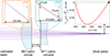 |
Figure 5 Illustrative ray-tracing of a the two lens achromat consisting of a positive and negative lens fulfilling the goal for achromatism (I) that was estimated with paraxial theory. |
This observation leads to the idea, that for certain combinations of positive and negative dispersing optical elements, the derived paraxial equations are still valid and useful. Therefore, we suggest the introduction of a new discriminator ϵ: (12)
(12)
This discriminator is built on the idea to sum the optical powers to a single value. A higher optical power, positive or negative, has stronger positive or negative dispersion. It then is multiplied by the ratio of partial dispersion and the Abbe number to weight the dispersion of longer wavelengths stronger, as the reversal of their chromatic dispersion is harder within the visual spectrum. This is caused by the smaller slope of the refractive index of typically used glasses. For infrared light and diffractive optical elements this does not apply.
The factor sRef in equation (12) is a reference length for normalization of the optical power. It should be adjusted to the expected lens thickness. In this article sRef = 1 mm is used, because of the given design volume. It may also become sRef = si for more accurate results, but then cannot be estimated a priori.
The discriminator should be kept sightly below zero ϵ ≤ 0. This ensures, that there is sufficient negative dispersion to compensate the later in the design process introduced lens thickness. However, there also should not only be negative dispersion present in the system. For the chosen sRef = 1 mm, a lower limit of ϵ > −1 × 10⁻³ is not advisable to be crossed. Applied to the in this article discussed two-lens examples, the resulting ϵSF11,SF11 = 1 × 10⁻⁴ (comp. Appendix A.2) and ϵBK7,SF11 = −4.4 × 10⁻⁵ (see Fig. 5) accurately distinguish the two cases. The former does not provide sufficient negative dispersion and therefore, the paraxial calculations may not be trustworthy. The latter, fulfills the requirements and it can be assumed, that the paraxial calculations may form a sufficient accurate start system for further optimization. This is confirmed by the ray-tracing in Figure 5.
2.2 Design of a three-lens system
Based on the introduced equations and estimators, it can be derived, that a system of three refractive lenses has sufficient free parameters to achieve the primary goals (I) and (II). Following the systematic approach, it may be separated into a collimation subsystem consisting of a negative and a positive lens and a second focusing subsystem consisting of a single positive lens. In order to maximize demand (II) for the secondary spectrum, the subsystem should be chosen accordingly. As this cannot be simply derived from νi and pi of the individual lenses, a new quantity ξ1,k to characterize the secondary dispersion of a system of k lenses shall be introduced: (13)
(13)
For single lens this equation simply represents the ratio ϱ/ν, just as used formerly in equation (12). At first, the two-lens collimator shall be designed with these paraxial estimations. The distance between the two lenses s2 thereby must meet the collimation condition. Therefore, it can be estimated as: (14)where θ1 = arcsin(NAF) is the aperture angle of the common fiber and D2 the desired diameter of the collimated output beam. Using
  for this estimation represents the compromise for exposure and measurement wavelength, λF and λC, respectively. Analogously, the first distance to the fiber facet can be derived. With insertion of equation (14) follows:
 (15)
(15)
Thereby,  can be expressed as focal length of the collimator sub-system. s1 and s2 now control the parameter space of suitable focal lengths of the two lenses. For s1, s2 > 0, the two ranges to attain the combination
  ,
,  can be found as:
 (16)
(16)
![Mathematical equation: $$ -1/[1/{f}_{\mathrm{1,2}}^d-1/{f}_2^d]<{f}_1^d<0. $$](/articles/jeos/full_html/2025/01/jeos20250010/jeos20250010-eq26.gif) (17)
(17)
Opposite to  ,
,  , this case minimizes the total sub-system length s1 + s2. Using these equations, a collimator sub-system with a targeted D2 = 4 for a common fiber NAF = 0.12 is directly fixed as
  . The subsystem is estimated to consist of two stock lenses with
  and
and  mm, respectively. Given these, different material combinations can be analyzed to maximize the secondary system dispersion ξ1,2. Figure 6 shows these for the materials given in Table 1. For given available fiber-coupled laserdiodes, λF = 448 nm, λC1 = 642 nm, and λC2 = 662 nm are picked for the design. Combinations of strong dispersive with low dispersive glasses exhibit stronger dispersion for longer wavelengths. It is possible to achieve negative dispersion for combinations of low dispersion with high dispersion glasses. However, this might be reversed by the later added third focusing lens.
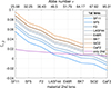 |
Figure 6 System dispersion of the first two-lens subsystem. |
To judge whether achromatism for goal (I) is achievable, Figure 7 shows the from equation (12) calculated reliabilities ϵ1,2. Green color marks a sufficient negative dispersion for a safe estimation, while red values probably will not result in a viable solutions. It is confirmed, that the first negative lens should be of highly dispersive glass to ensure a safe estimation. Accordingly, the first lens should be made of SF11. For the second lens, all other glasses might be of interest for the whole system. These shall be further investigated and combined with the third focusing lens.
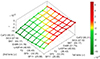 |
Figure 7 Paraxial estimation reliabilities ϵ1,2 for the dispersion of the two-lens subsystem. |
As the distances s1 and s2 are already fixed by the collimation criteria, the third lens must enforce the primary goal (I). For this purpose it is efficient, to use the recursive variant of equation (10), similar to equation (5): (18)
(18)
Thereby  is the two-lens collimator sub-system. Its t2 is described by equation (6). Inserting goal (I) and transforming for s3, yields the searched distance for an achromatic paraxial result between λF and λC:
 (19)
(19)
For a desired (reverse) magnification of the three-lens system of M > 1×, a suitable focal length for the third stock lens could be  . For an desired Airy disc of d
F ≈ 3 μm for the exposure, this requires a collimated beam diameter of D2 ≥ 4 mm. Applying now equation (19), should result in paraxial systems fulfilling primary goal (I). To maximize the second primary goal (II), Figure 8 shows the expected secondary spectra. Thereby, the calculated s3 ⊂ [28, 32] mm varied only within a small range. Surprisingly, goal (II) will be significantly better fulfilled, if the second lens is of a medium dispersive material, here: LASF44 and E48R. Regarding the material choice of the third lens it is implied by Figure 8, that a highly dispersive glass would be good. Applying the reliability estimator ϵ1,3 equation (12) again, reveals the safer estimations from the paraxial calculation. Figure 9 shows, that for the interesting collimator combination SF11 & E48R, a reliable start system can only include a third lens of E48R, BK7 or SiO2.
. For an desired Airy disc of d
F ≈ 3 μm for the exposure, this requires a collimated beam diameter of D2 ≥ 4 mm. Applying now equation (19), should result in paraxial systems fulfilling primary goal (I). To maximize the second primary goal (II), Figure 8 shows the expected secondary spectra. Thereby, the calculated s3 ⊂ [28, 32] mm varied only within a small range. Surprisingly, goal (II) will be significantly better fulfilled, if the second lens is of a medium dispersive material, here: LASF44 and E48R. Regarding the material choice of the third lens it is implied by Figure 8, that a highly dispersive glass would be good. Applying the reliability estimator ϵ1,3 equation (12) again, reveals the safer estimations from the paraxial calculation. Figure 9 shows, that for the interesting collimator combination SF11 & E48R, a reliable start system can only include a third lens of E48R, BK7 or SiO2.
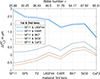 |
Figure 8 Dispersion of the three-lens system. |
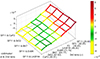 |
Figure 9 Paraxial estimation reliabilities ϵ1,3 for the dispersion of the three-lens system. |
According to Figure 8 should BK7 and SiO2 yield a slightly higher secondary spectrum, which should be advantageous for primary goal (II). However, the in the next design step added thickness of the lenses should be accounted for. This will enlarge the axial chromatic aberration significantly. Additionally considering the cost and weight of the system, the plastic E48R offers an attractive compromise. The paraxial design estimation therefore concludes with a start system consisting of a combination of a negative SF11 and two positive E48R lenses.
2.3 Ray-tracing optimization
Based on the designed start system, the more rigorous geometrical ray-tracing simulation and optimization of the system shall be performed. Therefore, real stock lenses of Table 1 are considered. The chosen three lenses are listed in Figure 10. Given the limited availabilities for stock optics, their focal length vary slightly from the paraxial design.
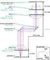 |
Figure 10 Via ray-tracing optimized three lens system with turning optics. |
The resulting axial chromatic aberration for a lens system with lenses at the paraxially estimated distances s1, s2 and s3 is shown in Figure 11 as turquoise initial curve. The start system nearly can achieve primary goal (I), but for a deviation of 20 μm. To eliminate this deviation, the multi-objective optimizer of the commercial ray-tracing software is employed [56]. With a heavier weight on the objective to eliminate axial color between λF and λC, solely the axial distances between the three lenses has been optimized. The optimized axial chromatic aberration in Figure 11 shows its resulting curve, that now achieves primary goal (I).
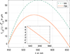 |
Figure 11 Chromatic focal shift of ray-tracing simulations before and after numerical optimization. |
Regarding primary goal (II), the inset in Figure 11 shows the magnified relevant range for the two focal planes of the measurement wavelengths. The two resulting defocii are zD1 ≈ 6 μm and zD2 ≈ −4 μm. These exceed the paraxially estimated maximized defocii in Figure 8 by far. The thereby effective  is estimated from the resulting lateral spot as
  . Using equation (1), this results in estimated normalized axial defocii of uD1 = 6.76 and uD1 = −4.51. Their average of
  thereby lies very close to the optimal value of uD,opt = 5.61 for ideal signals. The asymmetric distribution around the achromatic plane will take effect as a shifted working point on the differential curve.
Besides this axial chromatic behavior, this simple beam-path achieves a lateral Airy radius of r F ≈ 1.1 μm according to the ray-tracing software. This is below the nominal Airy disk of the third lens for an input beam of D2 ≈ 4 mm. For the medium measurement wavelength follows r C ≈ 1.66 μm. Therefore, the simulated system is considered optimized. For the actual measurement wavelengths that are focused on the defocused planes, the Airy radii r C1 ≈ 2.77 μm and r C2 ≈ 3.89 μm are slightly larger. This lateral widening indicates also an axial widening of the confocal peaks.
With this result, the optical design of the combined exposure and chromatic differential confocal measurement through a common fiber is finished. It marks a first example for the proposed design methodology for such systems.
3 Realized integrated tool head
As indicated in Figure 10, the beam-path features additional functions to enhance the usability and the ability to adjust to the local surface slope of the substrate. The main beam-path is folded by two 90° deflections due to space restrictions. For the first deflection a beam-splitter is inserted to integrate a camera chip. This 2D-array detector is observing the deflection of the beam to provide a feedback signal for the rotational NPMM-5D axes.
The movement of the spot on the camera is evaluated via the application of a threshold and a following centroid algorithm [57]. This provides a very fast processing time. Thereby the calculations are performed on the basis of a reference sphere. Its apex defines the center pixels xpx,0, ypx,0 on the camera. The two required surface angles can now be derived from the shift of the light spot on the camera. For an ideal sphere and square pixels follows for the azimuthal angle φ: (20)
(20)
For the polar angle ϑ, the surface slope, follows for lateral positions xIM, yIM on an ideal reference sphere with the diameter D0 as measured by the length interferometers: (21)
(21)
However, the optical system towards the camera imposes its imaging characteristics. Therefore, the measured  is only a rough estimate, that can be normalized by the number of total pixels Npx to allow the calculation of the arcus sine:
 (22)
(22)
Equations (21) and (22) can now be compared for every lateral position deviating from the reference sphere apex. Now, a position-depending correction coefficient can be derived: (23)
(23)
After this characterization, the polar angle  can be reconstructed online and used for the control of the rotational axes of the NPMM-5D.
Another not negligible function is the navigation and overview of the user on the substrate. Although the fiber-coupled confocal signals can be used for the reconstruction of surfaces, users often face different substrates of various shapes. To find regions of interest on these, a wide-field observation should be integrated. The already for angular measurements integrated camera is employed for this task. A problem is, that a wide-field illumination is missing. Therefore, wide-field imaging is performed in a rough way via axially defocusing the substrate with the positioning stage. Through the third focusing lens, this results in a rough, yet useful, image of the specimen on the camera.
The schematic overview of the realized total system is shown in Figure 12. Besides the already discussed optical beam-path, the different colored wavelengths are combined into the common fiber via a wavelength division multiplexer. Since their wavelength are very close to each other, the measurement lasers are combined via 2 × 2 couplers. This also applies to the wavelength-specific photodetectors. They are spectrally distinctive via notch filters for the two employed wavelength. Normal photodiodes are employed for intensity detection. Current signals are amplified via circuits following the design of [58]. The signals are read by a lock-in filter greatly enhancing the SNR of the signals via demodulation with a reference oscillation [59]. This reference oscillation was given to the employed laserdiode drivers, modulating the driving current. To reduce cross-talk, both laserdiodes are modulated at different frequencies, fC1 = 150 kHz and fC2 = 200 kHz, respectively. The created amplitude modulation is demodulated with the dual-phase scheme as indicated by Figure 12. This eliminates sensitivity to phase fluctuations in the analog signals. The demodulated two signals were calculated to their difference Δ and sum Σ. These signals are then transferred with an output sample rate of fS = 10 kHz to the digital signal processor of the NPMM-5D. There, these two are calculated to the normalized FES, which is used for focus control on the z-axis. The control loops run at fcyl = 3 kHz.
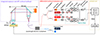 |
Figure 12 Schematic of designed optical measurement and exposure tool. |
The exposure laserdiode is monitored for power control via its own photodetector. A exposure dose controller directly modulates the laserdiode according to the scan speed of the spot on the substrate. A lock-in-filter is not implemented in order to achieve highest power stability for the exposure. The rotational axis will be controlled by the calculated polar and azimuth angle. Currently this evaluation has only been implemented offline. An online control loop is added in the near future.
4 Results
To demonstrate the integrated functions, several tests had been performed. For the larger part, the primary goals regarding the chromatic differential confocal measurement in conjunction with the exposure beam are confirmed. First, this measurement probe is characterized and, second, it is used for illustrative measurements. For another part, the integrated camera-based angular measurement is characterized.
4.1 Characterization of the differential confocal system
At first, it shall be investigated whether the design goals for the optical beam-path are fulfilled. Therefore a plane optical mirror is axially scanned through the focal planes. The z-axis is measured by the highly accurate interferometer. The individual confocal responses are shown in Figure 13. Visibly, the blue exposure laser has its focal plane between the two red measurement lasers. This confirms, that primary design goal (I) has been accomplished. The actual emission wavelength of both laserdiodes was determined to be slightly deviating to λC1 = 638 nm and λC2 = 658 nm, respectively. The axial defocii of the 638 nm-laserdiode and the 658 nm-laserdiode are zD1 = 8.7 μm and zD2 = −5.1 μm, respectively. Both values are close to the results from the ray-tracing optimization of zD1 ≈ 6 μm and zD2 ≈ −4 μm, but exceed them slightly. This may be caused by variation of the delivered lenses or the axial adjustment of the beam-path. Especially, the axial adjustment of the first negative SF11 lens has been identified as most sensitive. A larger distance towards the fiber facet will increase the axial separation of the response signals.
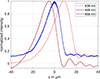 |
Figure 13 Measured axial response curves from a plane mirror. |
This eventually will come with the cost of widened spot-sizes on the specimen. To estimate the optimality of the adjustment, the full-width at half maximum of the response signals in Figure 13 can be evaluated via equation (1). For ideal sinc2() confocal signals [26], the normalized axial peak half-width is uHM = ±5.5662. From this, the effective NA may be estimated as NA F ≈ 0.22 and an average NA C ≈ 0.24. The former thereby results in an estimated Airy disk of r F ≈ 1.24 and thereby does not achieve the result from the ray-tracing resolution. The latter NAC exactly fits to the result from the ray-tracing optimization and therefore may result in the anticipated lateral spots. Given the manual adjustment procedure, this result therefore is considered as a sufficient precise adjustment.
Figure 14 shows the resulting differential curve Δ of the measurement signals. An asymmetry between negative and positive side can be observed. It stems from the already existing asymmetry of the confocal peaks from Figure 14 due to negative spherical aberration. It is caused by the first lens. The differential curve in Figure 14 had been derived from double-sided 30 repetitions over half an hour. From a moving window of N = 200, the repeatability at the working point of the exposure focus is uΔ = 82.8 nm with an expansion coefficient k = 1.
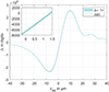 |
Figure 14 30× repeated measurement of the resulting differential curve. |
To reconstruct the actual depth, the relationship between the coaxial length interferometer and the non-ambiguous steep part of the differential curve Δ is approximated by analytical functions. Figure 15 shows the fit-result of three point-symmetric polynomials for the non-ambiguous region of Δ ⊂ [−15 × 103 dig,15 × 103 dig]. Clearly, the linearity on this range is limited. The maximum of the deviation  lies around the working point for the exposure laser. Therefore, higher polynomials are implemented into the control DSP of the NPMM-5D. For a fifth order polynomial, the maximum deviation is kept below
  . This is assumed to be sufficient, as the remaining oscillation is caused by a stick and slip behavior of the z-stage of the NPMM-5D.
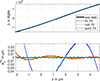 |
Figure 15 Fitted polynomials and residues within the working range of the differential signal. |
Mitigating this dynamic effect from the stage, Figure 16 shows step-movements in order to determine the axial resolution of the chromatic differential confocal probe. A flat mirror had been moved by 3 nm steps with a hold time of 10 s for each step. As there is only a single reflective interface involved, this is determining the single-surface resolution. As illustrated in Figure 16, the steps of 3 nm can be distinguished. Additional filtering with an ideal low-pass fC = 20 Hz emphasizes the attained axial single-surface resolution of the probe as shown by the dark-turquoise line.
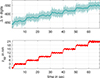 |
Figure 16 Demonstration of axial single-surface resolution of 3 nm of the differential signal (top) in comparison to the z-interferometer (bottom). |
However, the additional filtering also reveals aperiodic waveforms in the dark-turquoise line, that do not correlate with the stage movement as shown by the interferometer values below. These indicate the underlying instability of the fiber-coupled laserdiodes. Although the used laserdiodes are temperature- and current-controlled, chaotic de-stabilization from back reflection into the source appears. Note that these power uncertainties are below one percent. This unfortunately takes place in an unfavorable frequency space from approximately 0–1000 Hz. Thereby it overlaps with the measurement signal and cannot be removed with the lock-in filter.
4.2 Demonstration on reference targets
The shown axial single-digit nanometer resolution promises a very good performance for the accurate exposure focus control on pre-structured substrates. To test this ability, a lateral resolution reference target was measured. The SiMetrics RS-M was employed for this purpose. Its a bare silicon chip with various etched line gratings with pitches ϱ from 4 μm to 800 μm and a nominal depth of hRSM ≈ 3 μm. Measurements were performed orthogonal to the lines of the grating. Thereby, a closed loop measurement towards the surface was performed. This means that the signal of the chromatic differential confocal probe was directly used to move the axial stage back into the working point. Nevertheless, the axial stage still has an inner control loop where the interferometers provide feedback ([60], p. 135). The differential confocal signal had been used as slower outer feedback. As it is slower, it may not always be possible to move back into the working point of the differential probe during lateral scans. To compensate for this lag, the characterized non-ambiguous range was used to calculate correct depth values during movements: (24)
(24)
Figure 17 shows the result on the grating with the nominal pitch of pnom = 80 μm in comparison to a measurement of a large range prototype for atomic force microscopy (AFM) [61, 62]. Both measurements are area scans that were performed approximately in the same region on the line grating. These area scans then were corrected for their respective slant and rotation. In the end, the area scan was flushed into its projection on the xz-plane by taking the average along the y-direction.
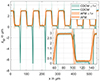 |
Figure 17 Measured profile of the pnom = 80 μm line grating in comparison to a long range AFM measurement. |
Visibly, the chromatic differential confocal measurement in Figure 17 exhibits large signal peaks at the edges of the structure. These are caused by the diffraction of the coherent focused measurement leasers. Typically, these so called bat-wings are symmetrical towards the grating [63, 64]. However, the here found asymmetry suggests, that the specimen is slightly tilted, because one side of the trench can be measured well. On the other side of the trenches, the about 7 μm deep diffraction minima are amplified by the shadow of the structure.
Comparing the result to the AFM-measurement, both confirm each other well. Of special importance is the height measurement in order to demonstrate a correct height reconstruction. The wide plateaus of the pnom = 80 μm will be evaluated to prevent the diffraction to affect this height measurement. Relevant height data is identified through the diagrams histograms. The chromatic differential confocal measurement reconstructs an average hCDCM = 2.769 ± 0.212 μm, k = 1 while the AFM provides hAFM = 2.687 ± 0.129 μm, k = 1. As the uncertainty region of one measurement includes the average value of the respective other measurement, this comparison implies an accurate height reconstruction for flat specimen regions. The major contributor to this uncertainty is the specimen itself. The chromatic differential confocal probe exhibits higher uncertainty due to the power fluctuation from the two laserdiodes.
The pitches of the two measurements pCDCM = 79.714 ± 0.695 μm, k = 1 and pAFM = 79.956 ± 0.406 μm, k = 1 align well. The inset in Figure 17 shows a single period and the critical dimension. The latter is warped by the diffraction effect and cannot be clearly derived. Overall, the pnom = 80 μm line grating is clearly resolved by the chromatic differential confocal probe. With expected Airy disks for the measurement focus of r C ≈ 1.64 μm, the pnom = 4 μm grating should be resolved. Indeed, the spatial Fourier transforms of the respective line grating measurement shown in Figure 18 reveal significant peaks at the nominal pitches of the SiMetrics RS-M.
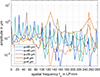 |
Figure 18 Spatial Fourier transform of measured line gratings on SiMetrics RS-M. |
The peak at fx = 250 LP/mm in Figure 18 confirms sufficient imaging contrast for the smallest grating. The actual profile measurement is shown in Figure 19. Visibly, the pitch of the grating can be derived, but the height is not accurate anymore. The depth of the grating is considerably too large. AFM measurements disprove this. This is caused by the merging diffraction effects of the grating onto chromatic differential confocal signals. For the special case of an approximately rectangular linear grating, the smallest pitch offering a plateau for height measurements was pnom = 20 μm.
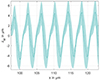 |
Figure 19 Measured profile of the pnom = 4 μm line grating. |
The shown resolution tests and demonstration on an rectangular grating proof, that the developed exposure and measurement tool can deal with non-continuous substrate surfaces in certain limits. If the non-continuous edge is interpreted as a very steep slope, the question arises, what is the maximum slope the tool can follow in closed loop mode. This especially regards continuous free-form substrates. For this purpose, a reference sphere shall be examined. Closed loop profile measurements radially across the apex of a D0 = 8 mm steel sphere are shown in Figure 20. Different lateral scan velocities vx ⊂ {5 μm s−1, 10 μm s−1, 20 μm s−1} were tested. It can be seen that the slowest scan velocity leads to the earliest surface loss. For vx = 5 μm s−1 the maximum surface angle can be calculated via equation (21) as  , while for vx = 20 μm s−1 a
  can be reached.
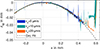 |
Figure 20 Measurements on reference sphere in closed-loop mode under different scan velocities. |
This effect can be explained with the dynamics of the control structure. The outer control loop incorporating the signal is too slow to follow the fast height changes that suddenly appear during the faster lateral movement. The employed sphere is not perfect and contains local trenches and humps. As these appear for all tested velocities, it is deduced, that these are real objects. Here the filter behavior of the outer control loop can be observed as smaller local peaks for higher velocities in Figure 20. As the NPMM-5D follows these local peaks and slopes further for the slow vx = 5 μm s−1, this local slope causes it to lose the surface for lower angles. This local slope then exceed the maximum angle only for a short lateral distance. The higher velocities there can jump over this local slope, until they lose the signal as well.
It however can be assumed, that an angle of ϑmax = 8° can be achieved for the scan of free-form surfaces. As seen in Figure 20 for larger positive distances for vx = 20 μm s−1, significant systematic deviations from a fitted reference circle may appear for the measurement signal on higher surface tilts. These stem from the dynamically changing aberration the reflected beam inherits after reflection towards the common fiber. This effect had been studied elsewhere [65, 66] and will lead to a defocus of the exposure tool on free-form substrates with steep slopes.
4.3 Angular measurements
The identified limits of the chromatic differential confocal measurement regarding the surface slope are now even more motivating for the ability of the tool to align its axis perpendicular to the local surface slope. The proposed angular measurement beam-path can provide the two necessary feedback signals φ and ϑ.
In order to characterize the angular measurement, the reflected spot image of the reference steel sphere was evaluated for a rectangular grid of lateral positions. The sphere apex was determined before by confocal measurements and is in center of the probed grid. For each lateral position, an axial stack of 15 images in steps of Δz = 20 μm was taken. For each image the spot center is determined by the aforementioned centroid algorithm. An average center position is determined from all 15 respective centers. The procedure ensures, that angles can constructed from defocus positions, too. This is relevant for the previous situation when the confocal signal leads to a defocus position due to the surface curvature or signal loss.
Figure 21 shows the with equation (20) reconstructed azimuthal surface angle and its residues from the ideal the ideal arctan2()-reference plane for all 360°. For large angles, the observed spot on the camera is cut off, because of the limited size of the sensor. Significantly, the discontinuity of the arctan2() leads to a high sensitivity for small deviations of the reconstructed spot center for small angles. Assuming a static relationship for systmatic deviations, a surface polynomial was fitted and subtracted from the measurements. This leads to a remaining standard deviation for the reconstructed azimuthal angles of σα,RMS = 0.1° as shown in Figure 21. For small angles the uncertainty remains higher due to the discontinuity.
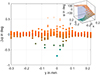 |
Figure 21 Projection of residual deviations for the azimuthal angular measurement. The inset shows the absolute azimuthal angle compared to the reference light-blue tangens-spiral. |
For the polar angle, Figure 22 shows the resulting reconstructed cone characterizing the local steepness of the substrate. The resulting αM were calculated from equation (23). Surface slopes up to ϑmax ≤ 6° can be acquired. Higher surface slopes lead to higher deviations from the reference arcsin()-plane. A surface polynomial had been subtracted to account for static systematic deviations, too. A remaining standard deviation of σϑ = 0.46° can be determined for the whole range as shown by the projection in Figure 22. This deviation significantly improves to σϑ = 0.16° for small surface slopes of ϑ ≤ 1°.
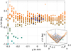 |
Figure 22 Projection of residual deviations for the polar angular measurement. Blue circled points are below 1° tilt. The inset shows the absolute polar angle compared to the reference light-blue sine-cone. |
The improvement for smaller surface slopes fits to the target function to adjust the tool axis perpendicular to the local slope. It is not necessary to have a very precise signal for larger surface slopes, as long as it can be used to lead back to the more precise center measurement. Currently, the major contributor to systematic and random deviations is the spot on the camera itself. By aiming for higher resolution, the beam of about D2 ≈ 4 mm is imaged onto the camera chip. Thereby, interference patterns from the coherent laserdiodes are visible. These patterns are very sensitive to vibration and small surface features such as roughness. For the applied thresholding and centroid calculation this leads to shifts of the reconstructed centers, which subsequently lead to deviations for the reconstructed angles.
5 Discussion
The performed tests and their results confirm the successful integration of surface focus- and angular-control into a small optical exposure and measurement tool head. Thereby, the angular measurement with the evaluation of a highly coherent spot shows good robustness against axial defocus from the surface. This also stems from the axially separated focii of the red measurement lasers that are used for the angular measurement. Although the overlay of these two beams leads to a higher temporal incoherence, the resulting image still shows significant coherent diffraction patterns. Finding a common robust threshold for these turned out to be not feasible. Therefore, it is anticipated, that the angular measurement would improve drastically by adding another tube lens into the camera beam-path (comp. Fig. 12). The camera does not necessarily need to be in this lens’ focal plane, but only requires a smaller spot on the camera. This enlarges the angular measurement range and improves the angular resolution. The latter profits from a higher spatial incoherence and under-sampling of the diffraction pattern by the finite camera pixels.
Regarding the chromatic differential confocal measurement setup, the new design methodology has been proven useful. The setup shows single-digit axial resolution from a compact beam-path. This axial resolution was anticipated to be higher, because of the integrated lock-in-filters and the realized beam-path with axial confocal defocii close to the assumed optimum. For the simple difference Δ aperiodic signal fluctuations prevent higher axial resolution. Their origin lies within the employed fiber-coupled laserdiodes, as they are prone to back-reflections from e.g. their own fiber facet.
In other differential confocal setups, such power fluctuation can also appear. However, these setups usually only employ one light source. Subsequently, all defocused confocal detectors acquire the same fluctuation. The FES of equation (2) then allows for ideal equal signal-processing, that these multiplicative disturbances are eliminated by normalization with the sum signal [33]. Here, this mechanism does not work, as two independently fluctuating laserdiodes are used for the calculation of the differential curve. This results in the aperiodic fluctuations that limit the axial resolution to 3 nm.
A possibility to improve this could be the integration of Faraday isolators to the beam path. Since the fiber-coupled laserdiodes’ own facet turns is causing the fluctuations, a shift to a free-space system with additional fiber-coupling would be necessary. An approach that aims for the use of fiber components might be the observation of the individual fluctuation. It could be included in the calculation of the FES. This would require additional observer photodiodes for each laserdiode that must be properly scaled for the integration with the signals detected from the specimen. This integration will be possible, as a growing number of laserdiodes include the photodiode on the same chip for optical power control application. Another approach could be the rewiring of the optical fibers, so that the opposite laserdiode’s detector can directly acquire the additional fluctuation. Proper signal scaling becomes more demanding in such an optical setup.
Additionally, the keen reader might have noticed, that the results for the chromatic differential confocal were only covered by Δ and not the FES, although the latter would be necessary for the elimination of the fluctuations. As it turned out, the sum signal Σ of the two confocal peaks is unfavorable for the normalization as illustrated by Figure 23. The resulting FES shows a reduced linearity and sensitivity for its lower part of the non-ambiguous range compared to the corresponding difference Δ. Even severe, the prominent minimum and maximum on the FES vanished. This results from the asymmetric shapes of the confocal response signals as seen in Figure 13. They cause a big widening of the signal Δ, especially for the values below the half maximum of Σ. Subsequently, the drop of the FES outside the non-ambiguous range is not reaching zero as ideally assumed, but lifted to a long tail for positive z-values. It may even be amplified at far away defocused positions as seen for negative z-values in Figure 23.
Although the non-ambiguous range has reduced sensitivity and higher non-linearity, it would still be usable for surface profilometry. It was tested, but was found to be too instable for surface scans on the shown specimen. Due to the axially separated focal planes the two measurement lasers are focused onto, the diffraction they are subjected to becomes different, too. As the working point is in between the two response peaks (comp. Fig. 13), the two unequal sides of the asymmetric depth responses are evaluated. This amplifies the different diffraction that is caused by the different focal planes on the specimen. In a third step, the calculation of the FES via equation (2) would lead to another amplification of the effect on the resulting differential curve via a distorted Σ in the denominator. This additional sensitivity by the denominator is implied by the higher non-linearity of the FES shown in Figure 23. The here observed effects thereby confirm the observations in [67] for a single source and wavelength.
Given this instability, the difference signal Δ solely was employed for surface profilometry in this article. This requires to perform characterizations on every specimen to account for their respective reflectivity and may lead to erroneous measurements when scanning over heterogeneous specimen. In order to incorporate this robustness in future chromatic differential confocal probes, the initially requested optimum axial separation of uD = 5.61 must be questioned. While this value may apply for detection paths, applying it to the illumination causes the described loss in robustness. This effect also leads to the significantly amplified diffraction effects in profile measurements as seen in Figure 17. If the two focal planes as well as the wavelength of the measurement beams are closer, their perceived diffraction becomes more similar. This would make the application of the FES possible again. The limiting case of this would be the use of the spectrum of a single laserdiode, which might also show more similar power fluctuation pattern for both signals.
6 Conclusion
This article introduced a new approach on the development of an integrated optical tool head for direct laser writing on curved substrates with the NPMM-5D. By incorporating axial and angular measurement, feedback signals are provided that allow the tool to be focused onto an unknown curved substrate, perpendicular to its local slope. The axial measurement thereby is realized as a chromatic differential confocal microscope. A new design methodology for the paraxial chromatic design was developed to find suitable initial systems that can combine exposure and measurement beams adequately. Here, the required achromatism between the exposure and the median measurement wavelength, but with a high axial chromatic separation for the two measurement wavelength, formed a special optical design goal. For this given use-case, this design methodology has proven useful for a three-lens design. It reduced the necessary experience from the designer and may speed up further designs. The design goal set for axial defocus between the measurement wavelengths could be achieved. Additionally, a long working distance of 6 mm had been realized.
The realized chromatic differential probe demonstrated axial resolution of 3 nm and a repeatability of 82.8 nm (k = 1). Height measurements on a reference target show well agreement to an AFM measurement. Regarding lateral resolution the probe with an average NA = 0.24 can provide contrast down to grating pitches of pnom = 4 μm. Due to diffraction effects of the nearly rectangular structure, these show no correct height measurement anymore. The smallest grating pitch that could show a plateau for height evaluation was pnom = 20 μm. Therefore, the application of the developed probe for profilometry on discontinuous substrates is limited. However, considering direct laser writing, continuous substrates are to be expected, where the diffraction effects become negligible.
It could be observed, that specimen induced diffraction in general is amplified by the axially separated measurement beams. Unfortunately, this meant that the supposedly more robust normalized focus error signal turned out to be instable on typical specimen. It is proposed to derive a new optimal defocus distance for chromatic differential confocal microscopes in the future to reduce this susceptibility to diffraction effects. Additionally, the design based on two independently fluctuating light sources, here two laserdiodes, reduces the stability of the differential curve and therefore is a major driver for the axial uncertainty, albeit the employed lock-in-filter. In future, these fluctuations might be compensated by additional observation principles or the reduction to a single light source.
The angular measurements for azimuthal and polar angle were realized by a camera observing the deflection of the nearly collimated reflected beam of the objective lens. Accounting for possible defocused positions of the tool head, the angular resolutions reach below 0.5° on a range from −66°. Given typical slants of supposedly flat substrates, this might be sufficient angular resolution for the approximate perpendicular adjustment on free-form substrates. Further improvement of angular range and resolution is expected by the introduction of another focusing lens that can reduce the spot size on the camera and the influence of interference pattern. A design rule for the optimum spot size should be found in the near future.
All in all, the realized integrated tool head already achieves more than sufficient resolution for following an arbitrary substrate surface with the exposure beam focus. It is considered ready for direct laser writing on free-form substrates and will therefore be integrated into the control structure and trajectory planner of the NPMM-5D in an upcoming development step.
Funding
This research was supported by the Deutsche Forschungsgemeinschaft (DFG) in the scope of the Research Training Group “Tip- and laser-based 3D-Nanofabrication in extended macroscopic working areas” (GRK 2182) as well as the transfer-project “Multiachs-Nanofabrikationsmaschine (MNFM)” at Technische Universität Ilmenau.
Conflicts of interest
The authors declare no conflict of interest.
Data availability statement
Measurement and simulation data is available upon reasonable request. Parts of the here shown data is only available in proprietary formats.
Author contribution statement
Johannes Belkner: Conceptualization, Methodology, Investigation, Formal analysis, Validation, Visualization, Writing – original draft, Johannes Leineweber: Conceptualization, Methodology, Investigation, Validation, Georg Hein: Investigation, Validation, Visualization, Data curation, Jaqueline Stauffenberg: Investigation, Formal analysis, Writing – review & editing, Alexander Barth: Conceptualization, Investigation, Thomas Kissinger: Conceptualization, Writing – review & editing, Eberhard Manske: Conceptualization, Methodology, Supervision, Funding acquisition, Writing – review & editing, Thomas Fröhlich: Methodology, Supervision, Funding acquisition, Writing – review & editing.
References
- Gissibl T, Thiele S, Herkommer A, Giessen H, Two photon direct laser writing of ultracompact multi-lens objectives, Nat. Photonics. 10, 554 (2016). https://doi.org/10.1038/nphoton.2016.121. [Google Scholar]
- Tsutsumi N, Hirota J, Kinashi K, Sakai W, Direct laser writing for micro-optical devices using a negative photoresist, Opt. Express 25, 31539 (2017). https://doi.org/10.1364/oe.25.031539. [Google Scholar]
- Qi H, Chen T, Yao L, Zuo T, Micromachining of microchannel on the polycarbonate substrate with CO2 laser direct-writing ablation, Opt. Lasers Eng. 47, 594 (2009). https://doi.org/10.1016/j.optlaseng.2008.09.004. [Google Scholar]
- Alsharhan TA, Young OM, Xu X, Stair AJ, Sochol RD, Integrated 3D printed microfluidic circuitry and soft microrobotic actuators via in situ direct laser writing, J. Micromech. Microeng. 31, 044001 (2021). https://doi.org/10.1088/1361-6439/abec1c. [Google Scholar]
- Teh KS, Additive direct-write microfabrication for MEMS: a review, Front. Mech. Eng. 12, 490 (2017). https://doi.org/10.1007/s11465-017-0484-4. [Google Scholar]
- Reeves JB, Jayne RK, Barrett L, White AE, Bishop DJ, Fabrication of multi-material 3D structures by the integration of direct laser writing and MEMS stencil patterning, Nanoscale 11, 3261 (2019). https://doi.org/10.1039/c8nr09174a. [Google Scholar]
- Moughames J, Jradi S, Chan TM, Akil S, Battie Y, Naciri AE, Herro Z, Guenneau S, Enoch S, Joly L, Cousin J, Bruyant A, Wavelength-scale light concentrator made by direct 3D laser writing of polymer metamaterials, Sci. Rep. 6, 33627 (2016). https://doi.org/10.1038/srep33627. [Google Scholar]
- Sakellari I, Yin X, Nesterov ML, Terzaki K, Xomalis A, Farsari M, 3D chiral plasmonic metamaterials fabricated by direct laser writing: the twisted omega particle, Adv. Opt. Mat. 5, 1700200 (2017). https://doi.org/10.1002/adom.201700200. [Google Scholar]
- von Freymann G, Ledermann A, Thiel M, Staude I, Essig S, Busch K, Wegener M, Three-dimensional nanostructures for photonics, Adv. Funct. Mater. 20, 1038 (2010). https://doi.org/10.1002/adfm.200901838. [Google Scholar]
- Hahn V, Kiefer P, Frenzel T, Qu J, Blasco E, Barner-Kowollik C, Wegener M, Rapid assembly of small materials building blocks (Voxels) into large functional 3D metamaterials, Adv. Funct. Mater. 30, 1907795 (2020). http://doi.org/10.1002/adfm.201907795. [CrossRef] [Google Scholar]
- An J, Le TSD, Lim CHJ, Tran VT, Zhan Z, Gao Y, Zheng L, Sun G, Kim YJ, Single-step selective laser writing of flexible photodetectors for wearable optoelectronics, Adv. Sci. 5, 1800496 (2018). http://doi.org/10.1002/advs.201800496. [Google Scholar]
- Liu W, Huang Y, Peng Y, Walczak M, Wang D, Chen Q, Liu Z, Li L, Stable wearable strain sensors on textiles by direct laser writing of graphene, ACS Appl. Nano Mater. 3, 283 (2020). http://doi.org/10.1021/acsanm.9b01937. [Google Scholar]
- Snow S, Jacobsen SC, Microfabrication processes on cylindrical substrates – Part II: Lithography and connections, Microelectron. Eng. 84, 11 (2007). https://doi.org/10.1016/j.mee.2006.06.009. [Google Scholar]
- Gehring H, Blaicher M, Grottke T, Pernice WHP, Reconfigurable nanophotonic circuitry enabled by direct-laser-writing, IEEE J. Sel. Top. Quantum Electron. 26, 1 (2020). https://doi.org/10.1109/jstqe.2020.3004278. [Google Scholar]
- Fendler C, Denker C, Harberts J, Bayat P, Zierold R, Loers G, Münzenberg M, Blick RH, Microscaffolds by direct laser writing for neurite guidance leading to tailor-made neuronal networks, Adv. Biosyst. 3, e1800329 (2019). https://doi.org/10.1002/adbi.201800329. [Google Scholar]
- Leineweber J, Hebenstreit R, Häcker AV, Meyer C, Füßl R, Manske E, Theska R, Charakterisierung eines parallelkinematisch aktuierten In-situ Referenzmesssystems für 5D-Nanomess- und Fabrikationsanwendungen, Technisches Messen. 91, 102 (2024). https://doi.org/10.1515/teme-2023-0109. [Google Scholar]
- Jäger G, Manske E, Hausotte T, Müller A, Balzer F, Nanopositioning and nanomeasuring machine NPMM-200 – a new powerful tool for large-range micro- and nanotechnology, Surf. Topogr. Metrol. Prop. 4, 034004 (2016). https://doi.org/10.1088/2051-672x/4/3/034004. [Google Scholar]
- De Groot P, Principles of interference microscopy for the measurement of surface topography, Adv. Opt. Photonics 7, 1 (2015). https://doi.org/10.1364/aop.7.000001. [NASA ADS] [CrossRef] [Google Scholar]
- Kim CS, Yoo H, Three-dimensional confocal reflectance microscopy for surface metrology, Meas. Sci. Technol. 32, 102002 (2021). https://doi.org/10.1088/1361-6501/ac04df. [Google Scholar]
- Podoleanu AG, Optical coherence tomography, J. Microsc. 247, 209 (2012). https://doi.org/10.1111/j.1365-2818.2012.03619.x. [Google Scholar]
- Wojtkowski M, Srinivasan VJ, Ko TH, Fujimoto JG, Kowalczyk A, Duker JS, Ultrahigh-resolution, high-speed, Fourier domain optical coherence tomography and methods for dispersion compensation, Opt. Express 12, 2404 (2024). https://doi.org/10.1364/opex.12.002404. [Google Scholar]
- Li J, Ma R, Bai J, High-precision chromatic confocal technologies: a review, Micromachines 15, 1224 (2024). https://doi.org/10.3390/mi15101224. [Google Scholar]
- Novak J, Miks A, Hyperchromats with linear dependence of longitudinal chromatic aberration on wave length, Optik 116, 165 (2005). https://doi.org/10.1016/j.ijleo.2005.01.003. [Google Scholar]
- Lu W, Chen C, Zhu H, Wang J, Leach R, Liu X, Wang J, Jiang X, Fast and accurate mean-shift vector based wavelength extraction for chromatic confocal microscopy, Meas. Sci. Technol. 30, 115104 (2019). https://doi.org/10.1088/1361-6501/ab2eab. [Google Scholar]
- Gu M, Sheppard CJR, Gan X, Image formation in a fiber-optical confocal scanning microscope, J. Opt. Soc. Am. A. 8, 1755 (1991). https://doi.org/10.1364/josaa.8.001755. [Google Scholar]
- Wilson T, Sheppard CJR, Theory and practice of scanning optical microscopy, 1st edn. (Academic Press Inc. Ltd, 1984). https://doi.org/10.1002/crat.2170201211. Available at https://www.researchgate.net/publication/234419246_Theory_And_Practice_Of_Scanning_Optical_Microscopy (accessed on: 2018 Mar 29). [Google Scholar]
- Mastylo R, Manske E, Jäger G, Entwicklung eines Fokussensors und Integration in die Nanopositionier und Nanomessmaschine (Development of a focus sensor and its integration into the nanopositioning and nanomeasuring machine), Technisches Messen. 71, 596 (2004). https://doi.org/10.1524/teme.71.11.596.51377. [Google Scholar]
- Wang Y, Liu J, Tan J, Differential confocal microscopy, in Confocal microscopy, in edited by J. Liu, J Tan (Morgan Claypool Publishers, 2016), p. 1–8. https://doi.org/10.1088/978-1-6817-4337-0ch7. [Google Scholar]
- Shimizu Y, Maruyama T, Nakagawa S, Chen YL, Matsukuma H, Gao W, A PD-edge method associated with the laser autocollimation for measurement of a focused laser beam diameter, Meas. Sci. Technol 29, 074006 (2018). https://doi.org/10.1088/13616501/aac0a6. [Google Scholar]
- Dinh VH, Hoang LP, Vu YNT, Cao XB, Auto focus methods in laser systems for use in high precision materials processing: a review, Meas. Sci. Technol. 167, 107625 (2023). https://doi.org/10.1016/j.optlaseng.2023.107625. [Google Scholar]
- Mastylo R, Dontsov D, Manske E, Jager G, A focus sensor for an application in a nanopositioning and nanomeasuring machine, in Optical Measurement Systems for Industrial Inspection IV, vol. 5856, edited by W. Osten, C. Gorecki, E.L. Novak (SPIE, 2005), p. 238. https://doi.org/10.1117/12.612887. [Google Scholar]
- Tan J, Wang F, Theoretical analysis and property study of optical focus detection based on differential con focal microscopy, Meas. Sci. Tech. 13, 1289 (2002). https://doi.org/10.1088/0957-0233/13/8/317. [Google Scholar]
- Liu J, Tan J, Bin H, Wang Y, Improved differential confocal microscopy with ultrahigh signal-to-noise ratio and reflectance disturbance resistibility, Appl. Opt. 48, 6195 (2009). https://doi.org/10.1364/ao.48.006195 [Google Scholar]
- Dobosz M, Optical profilometer: a practical approximate method of analysis, Appl. Opt. 22, 3983 (1983). https://doi.org/10.1364/ao.22.003983. [Google Scholar]
- Wang T, Wang Z, Yang Y, Mi X, Ti Y, Wang J, A differential confocal sensor for simultaneous position and slope acquisitions based on a zero-crossing prediction algorithm, Sensors 23, 1453 (2023). https://doi.org/10.3390/s23031453. [Google Scholar]
- Belkner J, Hofmann M, Kirchner J, Manske E, Demonstration of aberration-robust high-frequency modulated differential confocal microscopy with an oscillating pinhole, in Optics and Photonics for Advanced Dimensional Metrology, edited by P.J. De Groot, R.K. Leach, P. Picart (SPIE, 2000). https://doi.org/10.1117/12.2555558. [Google Scholar]
- Zhao W, Tan J, Qiu L, Bipolar absolute differential confocal approach to higher spatial resolution, Opt. Express 12, 5013 (2004). https://doi.org/10.1364/opex.12.005013. [Google Scholar]
- Qiu L, Zhao W, Feng Z, Ding X, A lateral super-resolution differential confocal technology with phase- only pupil filter, Optik 118, 67 (2007). https://doi.org/10.1016/j.ijleo.2005.12.013. [Google Scholar]
- Tan J, Liu J, Wang Y, Differential confocal microscopy with a wide measuring range based on polychromatic illumination, Meas. Sci. Technol. 21, 054013 (2010). https://doi.org/10.1088/0957-0233/21/5/054013. [Google Scholar]
- Chen LC, Nguyen DT, Chang YW, Precise optical surface profilometry using innovative chromatic differential confocal microscopy, Opt. Lett. 41, 5660 (2016). https://doi.org/10.1364/OL.41.005660. Available from: http://ol.osa.org/abstract.cfm?URI=ol-41-24-5660 (accessed on: April 30, 2018). [Google Scholar]
- Chen LC, Chang YW, Li HW, Full-field chromatic confocal surface profilometry employing digital micromirror device correspondence for minimizing lateral cross talks, Opt. Eng. 51, 081507 (2012). https://doi.org/10.1117/1.OE.51.8.081507. [Google Scholar]
- Zhao W, Liu C, Qiu L, Laser divided-aperture differential confocal sensing technology with improved axial resolution, Opt. Express 20, 25979 (2012). https://doi.org/10.1364/oe.20.025979. [Google Scholar]
- Corle TR, Fanton JT, Kino GS, Distance measurements by differential confocal optical ranging, Appl. Opt. 26, 2416 (1987). https://doi.org/10.1364/ao.26.002416. [Google Scholar]
- Hausotte T, Gröschl A, Schaude J, High-speed focal-distance-modulated fiber-coupled confocal sensor for coordinate measuring systems, Appl Opt. 57, 3907 (2018). https://doi.org/10.1364/AO.57.003907. [Google Scholar]
- Kirchner J, Mastylo R, Gerhardt U, Fern F, Weidenfeller L, Sasiuk T, Manske E, Schienbein R, Hofmann M, Sinzinger S, Anwendungen eines fasergekoppelten chromatisch konfokalen Sensors in Nanopositionier und Nanomessmaschinen (Applications of a fiber coupled chromatic confocal sensor in nanopositioning and nanomeasuring machines), Technisches Messen 86, 17 (2019). https://doi.org/10.1515/teme-2019-0041. [Google Scholar]
- Belkner J, Beiträge zum Direktlaserschreiben auf gekrümmten Oberflächen, Doktoringenieur (Dr.-Ing.), Technischen Universität Ilmenau, 2024. https://doi.org/10.22032/dbt.64256. [Google Scholar]
- Dereniak EL, Dereniak TD, Geometrical and Trigonometric Optics (Cambridge University Press, Cambridge, UK, 2008). [CrossRef] [Google Scholar]
- Dobson SL, Sun PC, Fainman Y, Diffractive lenses for chromatic confocal imaging, Appl. Opt. 36, 4744 (1997). https://doi.org/10.1364/ao.36.004744. [Google Scholar]
- Cui CC, Li H, Yu Q, Ye RF, Design of adjustable dispersive objective lens for chromatic confocal system, Opt. Precis. Eng. 25, 875 (2017). https://doi.org/10.3788/ope.20172504.0875. [Google Scholar]
- Mitschunas B, Sinzinger S, Startsystemfindung von Zoomoptiken mit Hilfe der Ilmenauer Software PARAX, DGaO – Proceedings Erlangen-Nürnberg: Dt. Gesellschaft für angewandte Optik 118, P5 (2017). Available at https://www.db-thueringen.de/receive/dbt_mods_00032926. [Google Scholar]
- Kingslake R, Johnson RB, Lens design fundamentals (Academic Press, 2009). [Google Scholar]
- SCHOTT North America Inc, Optical glass data sheets, 2017. Available at https://refractiveindex.info/download/data/2017/schott_2017-01-20.pdf. [Google Scholar]
- Sultanova N, Kasarova S, Nikolov I, Dispersion properties of optical polymers, Acta Phys. Pol. A 116, 585 (2009). https://doi.org/10.12693/aphyspola.116.585. [Google Scholar]
- Malitson IH, Interspecimen comparison of the refractive index of fused silica, J. Opt. Soc. Am. 55, 1205 (1965). https://doi.org/10.1364/josa.55.001205. [NASA ADS] [CrossRef] [Google Scholar]
- Li HH, Refractive index of alkaline earth halides and its wavelength and temperature derivatives, J. Phys. Chem. Ref. Data 9, 161 (1980). https://doi.org/10.1063/1.555616. [Google Scholar]
- LLC Z, Zemax OpticStudio 15.5 SP2. SP2. Version February 8, 2016, 2000. Available from: www.zemax.com (accessed on 17 October, 2023). [Google Scholar]
- Anderson F, Real time, video image centroid tracker, Proc. SPIE 1304, Acquisition, Tracking, and Pointing IV (SPIE, 1990). https://doi.org/10.1117/12.2322200. [Google Scholar]
- Wallin A, One-Inch-Photodetector, GitHub Repository (GitHub, 2020). Available from: https://github.com/aewallin/One-Inch-Photodetector (accessed on 23 October, 2023). [Google Scholar]
- Principles of lock-in detection and the state of the art, Technical report (Zurich Instruments AG, 2016). Available from: https://ziweb4.zhinst.com/applications/principles-oflock-in-detection (accessed on 3 March, 2020). [Google Scholar]
- Hausotte T, in Nanopositionier- und Nanomessmaschinen : Geräte für hochpräzise makro- bis nanoskalige Oberflächen- und Koordinatenmessungen, Habilitationsschrift, Chapter 10 (Pro Business, Berlin, 2011), p. 127–139. ISBN: 9783868059489. Available from: http://d-nb.info/1014995019. [Google Scholar]
- Stauffenberg J, Ortlepp I, Belkner J, Dontsov D, Langlotz E, Hesse S, Rangelow I, Manske E, Measurement precision of a planar nanopositioning machine with a range of motion of Ø100 mm, Appl. Sci. 12, 7843 (2022). https://doi.org/10.3390/app12157843. [Google Scholar]
- Stauffenberg J, Belkner J, Dontsov D, Herzog L, Hesse S, Rangelow IW, Ortlepp I, Kissinger T, Manske E, Investigations on tip-based large area nanofabrication and nanometrology using a planar nanopositioning machine (NFM-100), Meas. Sci. Technol. 35, 085011 (2024). https://doi.org/10.1088/1361-6501/ad4668. [Google Scholar]
- Xie W, Transfer characteristics of white light interferometers and confocal microscopes, PhD thesis (Universität Kassel, Fachbereich Elektrotechnik / Informatik, Kassel, 2017). Available at https://urn.fi/urn:nbn:de:hebis:34-2017112353867. [Google Scholar]
- Pahl T, Hagemeier S, Bischoff J, Manske E, Lehmann P, Rigorous 3D modeling of confocal microscopy on 2D surface topographies, Meas. Sci. Technol. 32, 094010 (2021). https://doi.org/10.1088/1361-6501/abfd69. [NASA ADS] [CrossRef] [Google Scholar]
- Rahlves M, Roth B, Reithmeier E, Systematic errors on curved microstructures caused by aberrations in confocal surface metrology, Opt. Express 23, 9640 (2015). https://doi.org/10.1364/oe.23.009640. [Google Scholar]
- Belkner J, Ortlepp I, Gerhardt U, Manske E, Compensating aberration induced error in differential confocal microscopy, in Optical Measurement Systems for Industrial Inspection XII, vol. 11782, edited by Lehmann P, Osten W, Gonçalves AA (SPIE, 2021), p. 117820P. https://doi.org/10.1117/12.2592392. [Google Scholar]
- Qiu L, Liu D, Zhao W, Cui H, Sheng Z, Real-time laser differential confocal microscopy without sample reflectivity effects, Opt. Express 22, 21626 (2014). https://doi.org/10.1364/oe.22.021626. [Google Scholar]
Appendix A: Paraxial derivations
A.1 Optical power of a system on k lenses
Paraxial theory shall be used to estimate the axial chromatic aberration of a system of k lenses as shown in Figure 4. The basic paraxial imaging by a single thin lens is given by many textbooks as [47, 51]: (A.1a)
 (A.1b)
As illustrated by Figure 4, γ1 is the angle of incidence of a single ray on the first thin lens at the height h1. Φ is the power of said thin lens, the inverse of its focal length: (A.2)
(A.2)
It depends on the refractive index of the lens and therefore on the wavelength. This depends on the specific optical element. For example, a spherical lens can be described by the famous lensmaker equation.
For a sequential combination for the first two lenses in Figure 4, the optical power Φ1,2 of their combination shall be derived. For the first lens follows from equation (A.1a):
Inserting this into equation (A.1b) it yields:
Adapting again equation (A.1a) to find γ3, it becomes:
Dividing this by −h1 yields the the power Φ1,2 of the two-lens combination via equation (A.1a) and (A.1b) as also derived in ([47], p. 151):
This system’s image-side principal plane  is at an axial distance t1 from the second lens:
From these statements it can be deduced, that a sequence of k lenses can be always divided into a system of two lenses where the first lens is actually system of thin lenses characterized by  and its optical power Φ1,k.
Therefore, for an arrangement of k lenses as indicated by Figure 4, the power of the system from the first to the kth lens can be described in analogue manner to equations (A.1a) and recursively as: (A.3)which is used in this article as equation (5).
A.2 False-positives for two-lens achromats
A first benchmark for the suggested equations (10) and (11) shall be the design of a two-lens achromatic system. From equation (10) follows for the realization of the desired achromatism between λF and λC for the distance between the thin lenses: (A.4)
(A.4)
Note, that this equation deviates from the textbook version, e.g. found in ([47], p. 316), because the difference has not been approximated by a differential. Obeying this equation for s2 satisfying demand (I), the evaluation for suitable material combinations can be judged by the second primary demand (II). For two lenses, equation (11) becomes: (A.5)
(A.5)
Regarding the optical tool head, the exposure beam emitted by the common fiber must be collimated and focused onto the substrate. For two lenses, such a system could be a combination of f1 = 50 mm and f2 = 12.5 mm. Theoretically, this would achieve a four times minified image of the single mode fiber core. Figure A.1 shows the from equation (A.5) calculated secondary power shifts. As this should be a measure for demand (II), the shown values should correspond to the local slope at λC.
For verification of this, the graph for a first lens made of E48R shall be analyzed in detail. Figure A.2 is showing the paraxially calculated focal shifts for every wavelength for the combination of an E48R collimator with an objective made of the materials of Table 1. Indeed, the estimation of the slope at λC generally agrees with the estimation resulting from  . A detailed look reveals, that for material-combinations that produce a lower minimum than
  , the estimation may underestimate the numerically correct slope at λC. This miss-estimation could be compensated by changing λd to be closer to λC. However, this may disagree with the actual design wavelength of the stock lens. Furthermore, the underestimation is safer for the actual design, because demand (II) should be maximized. This may compensate the limitations of the applied paraxial estimation.
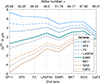 |
Figure A1 Secondary spectra of two-lens achromats. |
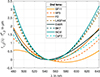 |
Figure A2 Chromatic focal shift for a two-lens Achromat with a first lens of E48R. |
As the keen reader now probably already found, the just shown results from two positive lenses are harboring an erroneous result for practical systems. In reality, two simple positive spherical lenses made of typical refractive material cannot fulfill the achromatic condition. This is because of the dispersion that appears due to the so far neglected thickness of the lenses. Especially for larger si, this results in large axial chromatic dispersion. Therefore, here the discriminator ϵ is introduced in equation (12) to judge the confidence about the paraxial estimation result.
All Tables
All Figures
|
Figure 1 CAD model view of the significant parts of the NPMM-5D. |
| In the text | |
|
Figure 2 Axial confocal response Iz and its sensitivity Sz, alias the differential confocal signal. |
| In the text | |
|
Figure 3 Target schematic of the optical tool, integrated with a chromatic differential confocal probe and its required axial chromatic separation of focal planes. Additionally, angular measurements are realized through a camera chip. |
| In the text | |
|
Figure 4 Schematic of paraxial ray crossing a system of k thin lenses characterized by their principal planes Pi, |
| In the text | |
|
Figure 5 Illustrative ray-tracing of a the two lens achromat consisting of a positive and negative lens fulfilling the goal for achromatism (I) that was estimated with paraxial theory. |
| In the text | |
|
Figure 6 System dispersion of the first two-lens subsystem. |
| In the text | |
|
Figure 7 Paraxial estimation reliabilities ϵ1,2 for the dispersion of the two-lens subsystem. |
| In the text | |
|
Figure 8 Dispersion of the three-lens system. |
| In the text | |
|
Figure 9 Paraxial estimation reliabilities ϵ1,3 for the dispersion of the three-lens system. |
| In the text | |
|
Figure 10 Via ray-tracing optimized three lens system with turning optics. |
| In the text | |
|
Figure 11 Chromatic focal shift of ray-tracing simulations before and after numerical optimization. |
| In the text | |
|
Figure 12 Schematic of designed optical measurement and exposure tool. |
| In the text | |
|
Figure 13 Measured axial response curves from a plane mirror. |
| In the text | |
|
Figure 14 30× repeated measurement of the resulting differential curve. |
| In the text | |
|
Figure 15 Fitted polynomials and residues within the working range of the differential signal. |
| In the text | |
|
Figure 16 Demonstration of axial single-surface resolution of 3 nm of the differential signal (top) in comparison to the z-interferometer (bottom). |
| In the text | |
|
Figure 17 Measured profile of the pnom = 80 μm line grating in comparison to a long range AFM measurement. |
| In the text | |
|
Figure 18 Spatial Fourier transform of measured line gratings on SiMetrics RS-M. |
| In the text | |
|
Figure 19 Measured profile of the pnom = 4 μm line grating. |
| In the text | |
|
Figure 20 Measurements on reference sphere in closed-loop mode under different scan velocities. |
| In the text | |
|
Figure 21 Projection of residual deviations for the azimuthal angular measurement. The inset shows the absolute azimuthal angle compared to the reference light-blue tangens-spiral. |
| In the text | |
|
Figure 22 Projection of residual deviations for the polar angular measurement. Blue circled points are below 1° tilt. The inset shows the absolute polar angle compared to the reference light-blue sine-cone. |
| In the text | |
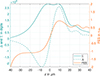 |
Figure 23 FES calculation from Δ and Σ corresponding to Figure 14. |
| In the text | |
|
Figure A1 Secondary spectra of two-lens achromats. |
| In the text | |
|
Figure A2 Chromatic focal shift for a two-lens Achromat with a first lens of E48R. |
| In the text | |
Current usage metrics show cumulative count of Article Views (full-text article views including HTML views, PDF and ePub downloads, according to the available data) and Abstracts Views on Vision4Press platform.
Data correspond to usage on the plateform after 2015. The current usage metrics is available 48-96 hours after online publication and is updated daily on week days.
Initial download of the metrics may take a while.