| Issue |
J. Eur. Opt. Society-Rapid Publ.
Volume 22, Number 1, 2026
Recent Advances on Optics and Photonics 2026
|
|
|---|---|---|
| Article Number | 27 | |
| Number of page(s) | 9 | |
| DOI | https://doi.org/10.1051/jeos/2026026 | |
| Published online | 23 April 2026 | |
Monte Carlo optimization for real-time magnetic domain learning in magneto-optical diffractive deep neural networks
Department of Materials Science and Bioengineering, Nagaoka University of Technology, 1603-1 Kamitomioka, Nagaoka, 940-2188, Japan
* Corresponding author: This email address is being protected from spambots. You need JavaScript enabled to view it.
Received:
13
December
2025
Accepted:
7
March
2026
Abstract
We propose an optimized algorithm using Monte Carlo Method (MCM) tailored for online learning in magneto-optical diffractive deep neural networks (MO-D2NN), a physical neural network platform where binary-weight are determined by magneto-optical modulation of light through the Faraday effect. Our derivative-free approach based MCM, iteratively adjusts the magnetic domain patterns to minimize cross-entropy loss without relying on gradients at a much lower computational cost. Our findings reveal that the MCM-based optimization algorithm serves as a robust and viable alternative to gradient descent-based training, achieving an accuracy of 96% for MNIST (Modified National Institute of Standard and Technology) handwritten digits classification with only a single hidden layer, highlighting its potential as a powerful approach for training MO-D2NN. We further validate its feasibility through physical implementation in an experimental optical setup, confirming its practical applicability for online image recognition tasks. We successfully demonstrate real-time learning of MO-D2NN using the MCM algorithm.
Key words: Monte Carlo optimization algorithm / Magneto-optical diffractive deep neural network / Image recognition / Online learning
© The Author(s), published by EDP Sciences, 2026
 This is an Open Access article distributed under the terms of the Creative Commons Attribution License (https://creativecommons.org/licenses/by/4.0), which permits unrestricted use, distribution, and reproduction in any medium, provided the original work is properly cited.
1 Introduction
The pursuit of ultrafast, energy-efficient computation has spurred renewed interest in physically implemented neural networks that operates beyond the limits of conventional electronic systems. Diffractive optical neural networks (D2NNs) process information across multiple layers by only passing light interacting with successive diffractive structures, achieving high-throughput inference at minimal power [1, 2]. Building on this foundation, magneto-optical D2NN (MO-D2NN) harness light propagation and interference while exploiting the Faraday effect in engineered magnetic thin films to encode binary weights as reconfigurable magnetic domains [3, 4]. This direct modulation of light through MO interactions provides intrinsic parallelism and low latency, allowing real-time neural computation at the speed of light. Such systems offer a compelling alternative to traditional electronic accelerators for tasks ranging from image recognition to language processing, and scientific computing. Despite their promise, the inability to update network parameters in real-time remains a major obstacle to the widespread deployment of physical neural networks. In most contemporary systems, neural networks are trained offline using numerical simulations, where stochastic gradient descent (SGD) methods such as backpropagation (BP) [5], are employed to minimize the loss function after which the optimized weights typically remain fixed. This approach significantly prevents real-time adaptation and limits performance in dynamic environments. The core limitation stems from the fundamental incompatibility between conventional gradient-based algorithms and the constraints of optical and hybrid neural systems. Such algorithms assume continuous, differentiable parameters, full observability, and deterministic behavior; conditions rarely met in practical optics, spintronics, or magneto-optics. Physical weights often require discrete or non-volatile updates, like magnetization switching, which are inherently non-differentiable. This highlights the need for efficient and compatible learning strategies tailored for physical implementations.
Monte Carlo methods (MCM) have a long legacy in physics and have demonstrated remarkable versatility across diverse scientific and engineering domains. Their applications extend from combinatorial optimization problems, such as scheduling and graph partitioning, to neural network optimization, and reinforced learning-based decision-making systems like AlphaGo [6]. They have also been widely employed within Nasa research, supporting Bayesian inference and state estimation with neural fields [7, 8], uncertainty quantification (UQ) in aerodynamic simulations [9], and recent Bayesian/UQ-initiatives aimed at assessing spacecraft performance under uncertainty and improving predictive modeling [10, 11]. By employing stochastic sampling with probabilistic acceptance, MCMs explore high-dimensional search spaces without relying on explicit derivatives. This makes them intrinsically compatible with the discrete, uncertain, and partially observable nature of physical neural systems. Their probabilistic structure also mitigates local minima, supports asynchronous updates, and minimizes unnecessary weight rewrites, key advantages for devices with limited endurance, like MO domain-switching networks. These features make MCM particularly well-suited for in-situ training, offering online adaptability and reconfigurability during operation, unlike conventional BP, which is generally limited to offline optimization and static inference.
This paper presents a theoretical framework of a Monte Carlo-based algorithm for online learning in MO-D2NN. The convergence behavior, classification performance on image recognition tasks (Handwritten digits, MNIST), and the underlying optimization strategy are examined through a generalized analysis. The proposed approach and its practical feasibility are confirmed were experimentally validated for online learning in MO-D2NN, as reported in our prior study [12]. The results provide new insights into Monte Carlo-driven physical neural networks and highlight its potential as a scalable scheme for next-generation neural computing. Although slower than conventional gradient-based methods in offline training, the approach is well suited to real-time physical implementation, where backpropagation cannot be directly applied. However, our research has primarily focused on MO-D2NN, where the proposed MCM-based learning has been validated, yet it is not restricted to MO-D2NN and can be extended to general diffractive deep neural networks (D2NNs). Because training relies exclusively on forward propagation combined with MCM updates, it is gradient-free and enables direct implementation in systems with discrete, or non-differentiable elements.
2 Monte Carlo optimization algorithmic approach
2.1 General MCM framework
Metropolis-inspired MCM optimization algorithm employed here is a gradient-free search strategy, in which binary weights of the diffractive network are iteratively updated through stochastic proposals and loss-guided acceptance. Each trainable configuration is represented by a binary weight vector v ∈ {−1, 1}N, where N denotes the number of trainable domains, as diffractive elements. The optimization of these binary weights is formulated as a stochastic search process directly guided by the system loss function. At each iteration, a new configuration v' is generated by flipping a predefined number of weight elements.
At each iteration, the optimization proceeds as follows:
- -
Initialization: The algorithm begins by randomly initializing a binary weight vector v(0) ϵ {0, 1}N, representing the initial magnetic domain configuration.
- -
Sampling generation: A new state v' is generated by flipping a subset of entries in the current magnetic domain in v, corresponding to local modifications of the domain configuration.
- -
Loss evaluation: The corresponding loss L(v') is computed by propagating the input through MO-D2NN and comparing the predicted distribution with the true label distribution. The change in loss in then obtained as:
- -
Acceptance rule: The update rule follows a deterministic Metropolis acceptance criterion. The candidate state is deterministically accepted if ∆L < 0, and the magnetic domain pattern is updated accordingly. Otherwise, the algorithm retains the previous configuration.


- -
Iteration and Termination: The steps of sampling, evaluation, and acceptance are repeated until convergence, or a predefined maximum number of iterations (MC-iterations) is reached, hereafter referred to as Nmax.
The efficiency of MCM optimization depends on its ability to explore the weight configurations within the hidden layer, which grow exponentially with network size. At each iteration, the network processes input data, computes the loss relative to the target, proposes random domain updates in the magnetic-optical layer, and applies weight flips to generate candidate configurations aimed at reducing the loss. Candidate configurations are accepted or rejected according to a Metropolis criterion, enabling derivative-free optimization (see the conceptual flowchart, Fig. 1).
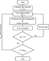 |
Figure 1 Algorithmic Flowchart of the employed MCM process. |
2.2 Application of MCM in practice
The MCM optimization was applied to train a fully connected MO-D2NN with binary phase encoded weights for image classification tasks. The network operates as a sequence of optical transformations, where each diffractive layer modulates the incident light. The resulting intensity distribution is measured at the output plane.
The forward light propagation was calculated numerically, accounting for the magneto-optical (MO) effect by separately propagating the right and left circularly polarized light. The MO effect, measured as polarization rotation and ellipticity, arises from differences in refractive index and extinction coefficient for the two circular polarizations. Free-space propagation was computed using the band-limited angular spectrum method [13], derived from the Rayleigh-Sommerfield diffraction formula [14], with Fourier-based convolutions, applying band-limiting and zero-padding to maintain sampling resolution and avoid aliasing.
The detector plane was partitioned into ten output regions arranged in three rows (3-4-3), corresponding to digit classes (0-9). The first, second, and third rows represent digits {0-2}, {3-6}, and {7-9}, respectively. Optical intensity was evaluated within these regions at the output plane, and the predicted digit was assigned to the region exhibiting the highest intensity. Classification was therefore performed using class-specific detectors associated with the target categories. During training, the MCM-algorithm iteratively adjusts the binary configuration of the magnetic domain pattern to minimize the classification error, evaluated through the cross-entropy-loss function comparing the predicted and target intensity distributions:
where C is the number of output classes, Qi(x) is the ground-truth one-hot label vector (the true class probability distribution), and ![Mathematical equation: $$ {P}_i\left(x;v\right)\in \left[0,1\right] $$](/articles/jeos/full_html/2026/01/jeos20250098/jeos20250098-eq7.gif) is the predicted class probability output for class i, under configuration v.
is the predicted class probability output for class i, under configuration v.
Through repeated stochastic updates and forward propagation calculations, the network converges toward a configuration that optimally maps the input to the desired output.
2.2.1 Network architecture
Calculations were performed using a single-layer MO-D2NN model shown in Figure 2, comprising N trainable neurons in a 100 × 100 neuron (1 μm width). Although the proposed training scheme is not restricted to a single hidden layer and has been numerically validated extensive simulations beyond the single-layer configuration, involving 2, 3, 4, 5, 10 and 15 diffractive layers, within the same training conditions, the MCM training jointly optimizes all layers simultaneously rather than sequentially optimizing each layer. However, deeper systems experimentally require significantly higher alignment precision and fabrication control. Therefore, for clarity and consistency with the online experimental study [12], we report computations for the single-layer configuration, which provide the theoretical foundation of our proposed approach. Diffractive layer was made from a perpendicular anisotropic magnetic material, with two out-of-plane magnetization domains σᵢ = ±1 (up or down), encoding phase shifts of 0 or π (+1 or −1), and updated via MCM. The network was driven by linearly polarized light at a wavelength of 532 nm. This wavelength was selected due to the strong magneto-optical response of bismuth-gallium substituted yttrium iron garnet (BIG), which served as the hidden layer in the network. BIG exhibits pronounced Faraday rotation in the visible spectral range, peaking near the green region around (532 nm) [12]. As reported in our previous study [15], the magneto-optical performance can be evaluated using the figure of merit (FOM), defined as the ratio of Faraday rotation relative to optical absorption, which quantifies the efficiency of polarization rotation to optical loss. At longer wavelength such as 633 nm, the Faraday rotation decreases due to the reduced MO response, optical absorption is also lower, resulting in higher transmittance and a comparable FOM. Consequently, the choice of 532 nm provides an optimal balance between maximizing Faraday rotation and minimizing optical loss, consistent with the intrinsic optical and MO properties of BIG films. The separations between the input-to-hidden layer (d1 = 3.0 mm) and between the hidden-to-output layer (d2 = 0.5 mm) were selected following an optimization of the inter-layer spacing, which identified 3.0 mm and 0.5 mm as the configurations yielding the highest accuracy. The refractive indices were set to n = 1 for free space and n = 2 for the substrate. Faraday rotation angle θF and the ellipticity ηF were assumed to be 3.3° and 0°, respectively, to maximize modulation and ensure optimal interaction with the magneto-optical layer. This configuration provides strong Faraday rotation while maintaining high optical transparency and stable diffraction patterns. To maintain consistency, the same polarization parameters were applied in both simulations and experiment. A polarizer oriented at 90° was placed between the last layer and detector, so that it was perpendicular to the polarization of the incident light.
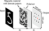 |
Figure 2 Structural overview of the MO-D2NN model featuring a single hidden layer and a polarizer. |
2.2.2 Datasets and task
Classification was performed on the MNIST handwritten digits dataset, with 5,000 training and 10,000 testing grayscale images of size 28 × 28. Each image was rescaled and rescaled to 100 × 100 pixels. Input images were propagated through the simulated optical network, and the output plane was segmented into ten-class specific detection areas corresponding to digits 0 ~ 9, each measuring 11 × 11 μm2. The predicted class was determined based on output plane intensity, providing a direct mapping from output pixels to their expected digit.
2.2.3 Loss function and evaluation
Convergence was tracked by loss reduction and test accuracy, with hyperparameters (flip size, iterations) set from preliminary runs. Loss was evaluated as the cross-entropy between target labels and normalized output intensities within each class regions, and classification accuracy was computed on the test set. Binary weights were updated via MCM proposals, accepting flips if loss did not increase or remained unchanged.
2.2.4 Training protocol
Training proceeded with fixed flip-size MCM updates, described above, for up to 80,000 iterations. At each step, a subset of binary weights awas proposed for flipping and loss was evaluated for both configurations. For each configuration we report convergence curves (loss vs iterations), and test accuracy vs. iterations. Optimization was entirely gradient-free, driven by stochastic binary search. Backpropagation baseline was included under identical data partitions for reference. When evaluating the loss, the algorithm computes ∆L, ensuring a consistent loss reduction without requiring explicit gradient computation.
2.2.5 Implementation details
Numerical simulations were conducted on a standard workstation-AI equipped with NVIDIA RTX-A6000 (48 GB of graphical processing unit-GPU, a Core i9-10980XE-18 cores / 36 thread of central processing unit-CPU, and 128 GB (32GB×4) of random-access memory-RAM), running on Ubuntu 20.04 LTS operating system. Python (v3.10.9), NumPy (1.23.2), and TensorFlow (v2.12.0) framework were used for most implementations. All experiments are repeated with multiple random seeds to insure statistical robustness.
2.3 Flip-size and initialization strategies in MCM optimization
To further investigate the impact of the initialization states and the update strategy on the optimization process, we evaluated multiple flip-sizes of the network weights. Initialization plays a key role in guiding the network toward optimal configurations, while the update strategy governs its exploration during each iteration. The choice of flip size shapes this process: smaller flips promote finer adjustments and more stable convergence, whereas larger flips enable broader exploration but may induce instability.
In this study, we examined two initialization configuration schemes:
- -
Deterministic initial state: where all the magnetic domains are initially aligned at the same direction (+1). Then number of weight flips were applied per iteration.
- -
Random initial state: where domains of the network are initialized stochastically at different directions (+1 or −1), following the same flip size sequence.
By systematically varying flip sizes (Fs = {1 × 1, 2 × 2, 3 × 3, 4 × 4, 5 × 5, 10 × 10 μm2}) within the two initialization states, we assessed their impact on convergence behavior, stability, accuracy, and overall performance. This analysis reveals the influence of the initial magnetic configuration on network performance and provides a comprehensive understanding on the interplay between initialization, update strategy, and flip size on convergence and optimization efficiency, offering valuable insights for selecting parameters that ensure robust network optimization.
3 Results and discussion
The performance of the MCM optimization was evaluated by comparing different fixed flip size strategies under different initialization configurations.
3.1 Effect of initialization and flip size on convergence
Figure 3 shows the evolution of training loss and accuracy convergence for deterministic and random initializations with a flip-size of 1 × 1 μm2 over the same number of iterations (80,000). In both cases, the loss decreased steadily without divergence, achieving monotonic or plateau-like loss reduction, consistent with the non-worsening acceptance rule that rejects unfavorable updates and allows equal-loss moves. However, their convergence characteristics differ underscoring the strong influence of initialization on MCM optimization.
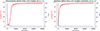 |
Figure 3 Classification accuracy and loss as functions of MC iterations for a fixed flip size of 1 × 1 μm2 under deterministic and random initial state. |
In the case of deterministic initialization, where all weights set to +1, loss exhibits a slower initial decrease in loss, reflecting its poor starting point far from an optimal weight configuration. The acceptance rate was initially low, and the network required more iterations before reaching stable convergence. Interestingly, in most trials, the network achieved a higher final accuracy of 96%, despite showing a transient peak in the very early stage (immediately after launch), followed by a slight decrease over 10∼ 50 iterations before resuming steady improvement. This indicates that although deterministic initialization suffers from a disadvantage at the beginning, the system can overcome its imbalance and eventually reach a strong performance.
Random initialization, where the weights are assigned randomly to ±1, shortens the computation time and yields to faster early convergence, the accuracy increases immediately, and the loss decreases without delay. In contrast, deterministic initialization requires more steps before any performance progress begins. Despite this efficiency advantage, the random scheme ultimately converges to a lower final accuracy (95%) than the deterministic one (96%). Comparing both configurations shows that each reaches a stable accuracy, with deterministic initialization converging more slowly but achieving a higher final accuracy, while random initialization accelerates the process with a modest reduction in final accuracy.
Increasing the flip size 1 × 1 μm2 to 10 × 10 μm2 destabilizes the optimization process, reducing accuracy and causing the loss divergence under deterministic initialization (Fig. 4). The observed instability originates from excessively large domain sizes, which reduce the number of neurons. The resulting performance degradation is therefore not an intrinsic limitation of the MCM-based learning scheme, but a consequence of the underlying update process, where larger flips induce stronger perturbations while simultaneously reducing the neuron counts, whereas smaller flips allow finer exploration of the configuration space and promote more stable convergence. Consequently, this behavior reflects an algorithmic trade-off between update step size, neurons number, and convergence stability, rather than a fundamental constraint of the method.
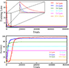 |
Figure 4 Training loss (top panel) and accuracy (bottom panel) versus the number of trials for various flip sizes under deterministic initialization. |
Figure 5 displays theoretical results for a sample input, obtained after optimization from a random initial state using a flip size of 1 × 1 μm2, and 80,000 MC iterations. The input image (a) is mapped through the trained domain distribution, revealing the magnetic domain pattern in the hidden layer (b), the output intensity (c), the masked detector-plane intensity (d), along with the corresponding classifier response. For a given input digit ‘5’, the classifier produces the highest activation for the correct label, matching the input, confirming that MCM effectively encodes input digits into distinct magnetic domain configurations for accurate digits recognition.
 |
Figure 5 Simulation results of digit ‘5’ with intensity detection and true class distribution. |
3.2 Magnetic domain evolution
Figures 6 and 7 present the magnetic domain patterns obtained after training with different flip sizes for deterministic and random initialization. Small flip sizes (panels a–c) produce well-defined magnetic domain patterns, indicative of stable learning dynamics, whereas larger flip sizes (panels d–e) progressively degrade the pattern resolution, reflecting reduced learning stability. At a flip size of 10 × 10 μm2, (panel f) the resolution collapses into enlarged domains, demonstrating instability driven by excessively large parameter updates. This agrees with the accuracy and loss curves, which likewise exhibit degraded performance at larger flip sizes.
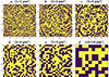 |
Figure 6 Magnetic domain patterns under random initial state, for flip sizes (a) 1 × 1, (b) 2 × 2, (c) 3 × 3, (d) 4 × 4, (e) 5 × 5 and (f) 10 × 10 μm2. |
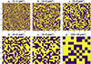 |
Figure 7 Magnetic domain patterns under deterministic initial state, for flip sizes: (a) 1 × 1, (b) 2 × 2, (c) 3 × 3, (d) 4 × 4, (e) 5 × 5 and (f) 10 × 10 μm2. |
Physically, this behavior originates from the diffraction-limited optical coupling condition, which governs light propagation between adjacent layers through its dependence on the diffraction angle (β) and the interlayer spacing. In a fully connected neural network, each neuron in one layer interacts with all neurons in the next. In an MO-D2NN, this connectivity is realized optically through the first-order diffracted light.
For a neuron of diameter dn, the 1st order diffraction angle β is given by:
From this angle, the interlayer distance ∆l needed to maintain full optical connectivity followed from the geometrical separation between the farthest neuron in adjacent layers:
where Nx and Ny are the numbers of neurons along the horizontal and vertical axes.
Our analysis shows that the input-to-hidden separation d1, evaluated over a range of values reveals d1 = 3.0 mm as providing optimal classification performance. With d1 fixed, varying the hidden-to-output spacing indicates that d2 = 0.5 mm optimizes both accuracy and loss convergence. Further analysis, with d1 fixed and d2 set according to the fully connected equation for different flip sizes (Fig. 8), showed that at non-optimal values, accuracy is only weakly affected by interlayer distance, whereas the number of neurons predominantly influences performance. These distances are consistent with diffraction-limited coupling, where first-order diffracted light efficiently transmits between layers.
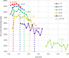 |
Figure 8 Accuracy as functions of the hidden-to-output layer separation d2 for different flip sizes, with the input-hidden spacing d1 fixed at 3.0 mm. |
3.3 Comparative insights into MCM and SGD-based BP
We evaluated both MCM and SGD with BP in terms of training loss under identical conditions on 5,000 training and 10,000 testing images. BP was trained for 50 epochs with a batch size of 50, totaling 5,000 trials in total, while MCM used the same training and testing sets over 80,000 iterations. As shown in Figure 9, MCM starts from higher initial losses, over 50 for deterministic initialization, and around 10 for random initial state. Whereas BP begins near 0.7 and converges faster per trial. Within the first trials, MCM reaches a loss profile nearly identical to BP, indicating that despite its slower start, it ultimately achieves comparable convergence. MCM theoretically requires more iterations (~ 80,000 trials) and about 20 hours, far exceeding BP, which completes the training in roughly 20 min.
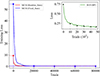 |
Figure 9 Loss convergence over 80,000 MCM trials for deterministic (blue) and random (red) initializations. Results are compared with a 5,000-trial BP baseline (inset, top-right). |
Crucially, MCM permits direct online adaptation within the physical system, an approach that is not accessible to BP owing to its reliance on gradient propagation and discrete activations. Using our optical platform, training was performed on a single-layer MO-D2NN. The experimental parameters were aligned with the theoretical computations outlined above, including the inter-layer distances (3.0 mm, 0.5 mm) and the image size (100 × 100 μm2), ensuring direct correspondence between simulation and implementation. Input images were generated by illuminating a linearly polarized laser beam (λ = 532 nm) onto a chromium-on-glass photomask fabricated via photolithography and maskless patterning (MX-1240, Japan Science Engineering Co., Ltd.), where handwritten digit patterns chemically etched. The bismuth-gallium-substituted yttrium iron garnet thin film, served as the hidden-layer owing to its large Faraday effect and high optical transparency. Magnetic domain was recorded using thermo-magnetic recording system. Detailed fabrication and full experiment procedures are provided in our previous report [12, 16–18]. After each MCM trial, the resulting optical distribution at the output plane was recorded and classification loss was evaluated. Domain updates were retained only upon reduction of the loss, leading to progressive improvement in recognition performance over successive iterations. Processing a single MNIST image required approximately 2 hours over 200 MCM trials under the initial configuration. In an enhanced experimental arrangement presently under active development, 10 images were processed in 4 hours across 1,500 trials, reflecting improved stability and throughput. Despite this progress, scaling to the full dataset remains time-intensive with the present system. Nevertheless, these findings indicate that MCM is intrinsically compatible with real-time physical implementation, whereas BP remains predominantly confined to offline computational optimization. With further optimization of the optical architecture, introducing high-speed polarized camera (HSPC) and digital micromirrors device (DMD), faster magnetic dynamic switching and improved detection, the online training in principle could be significantly accelerated to seconds or even nanoseconds, allowing 60,000 images to be processed within minutes, underscoring the potential of MCM-based optimization in physical and hybrid neuromorphic systems.
4 Summary
We introduced a new training algorithm based on Monte Carlo Method (MCM) optimization for online learning in magneto-optical diffractive integrated neural network (MO-D2NN) applied to image classification. This derivative-free approach enables efficient training in discrete, non-differentiable systems. By avoiding gradient computations, the network achieved consistent 96% accuracy in classifying handwritten digits. The MCM-based algorithm was successfully applied in an experimental setup, demonstrating the update of magnetic domains in real time. Our study establishes theoretical and practical benefits of MCM optimization, offering a scalable solution to the challenges of gradient free training. While the results are promising, further refinements are needed to accelerate learning, reduce training time, improve efficiency for more complex tasks, and strengthen scalability toward real-time next-generation optical computing.
Funding
This work has been supported by JSPS Grant-in-Aid Scientific Research JP23H04803.
Conflicts of interest
The authors declare no conflict of interest.
Data availability statement
The data supporting the findings of this study can be obtained from the corresponding author upon request.
Author contribution statement
Fatima Zahra Chafi conceptualized, drafted and edited the manuscript, Fatima Zahra Chafi, Tomonao Matsuya, Kanata Watanabe conducted the theoretical study, Hotaka Sakaguchi performed experiments, Takayuki Ishibashi reviewed and guided the analysis of the work, all authors discussed the results and approved the final version.
References
- Lin X, Rivenson Y, Yardimci NT, Veli M, Luo Y, Jarrahi M, Ozcan A, All-optical machine learning using diffractive deep neural networks, Science 361, 1004–1008 (2018https://doi.org/10.1126/science.aat8084. [Google Scholar]
- Chen H, Feng J, Jiang M, Wang Y, Lin J, Tan J, Jin P, Diffractive deep neural networks at visible wavelengths, Engineering 7, 1483–1491 (2021https://doi.org/10.1016/j.eng.2020.07.032. [Google Scholar]
- Fujita T, Sakaguchi H, Zhang J, Nonaka H, Sumi S, Awano H, Ishibashi T, Magneto-optical diffractive deep neural network, Opt. Express 30, 36889–36899 (2022https://doi.org/10.1364/OE.470513. [Google Scholar]
- Sakaguchi H, Fujita T, Zhang J, Sumi S, Awano H, Nonaka H, Ishibashi T, Development of fabrication techniques for magneto-optical diffractive deep neural networks, IEEE Trans. Magn. 59, 1–4 (2023https://doi.org/10.1109/TMAG.2023.32818.4210. [Google Scholar]
- Rumelhart DE, Hinton GE, Williams RJ, Learning representations by back-propagating errors, Nature 323, 533–536 (1986https://doi.org/10.1038/323533a0. [Google Scholar]
- Silver D, Huang A, Maddison CJ, Guez A, Sifre L, Driessche GD, Schrittwieser J, Antonoglou I, Panneershelvam V, Lanctot M, Dieleman S, Grewe D, Nham J, Kalchbrenner N, Sutskever I, Lillicrap T, Leach M, Kavukcuoglu K, Graepel T, Hassabis D, Mastering the game of Go with deep neural networks and tree search, Nature 529, 484–489 (2016https://doi.org/10.1038/nature16961. [Google Scholar]
- Course K, Nair PB, State estimation of a physical system with unknown governing equations, Nature 622, 261–267 (2023https://doi.org/10.1038/s41586-023-06574-8. [Google Scholar]
- Hao K, Bilionis I, Neural information field filter, Machine Learning (2024). https://doi.org/10.48550/arXiv.2407.16502. [Google Scholar]
- Mukhopadhaya J, Whitehead BT, Quindlen JF, Alonso JJ, Multi-fidelity modeling of probabilistic aerodynamic databases for use in aerospace engineering, arXiv (2019). https://doi.org/10.48550/arXiv.1911.05036. [Google Scholar]
- Lee S, Kitahara M, Yaoyama T, Itoi T, Latent space-based Bayesian approach to the NASA and DNV challenge 2025, Proc. Conf. (2025https://doi.org/10.3850/978-981-94-3281-3_ESREL-SRA-E2025-P8724-cd. [Google Scholar]
- Butler RW, Caldwell JL, Carreno VA, Holloway CM, Miner PS, DiVito BL, NASA Langley’s research and technology transfer program in formal methods, Proceedings of the Tenth Annual Conference on Computer Assurance (COMPASS’95), IEEE, 101–110 (1995). https://doi.org/10.1109/CMPASS.1995.521893. [Google Scholar]
- Sakaguchi H, Oya R, Sumi S, Awano H, Nonaka H, Chafi FZ, Ishibashi T, Development of online learning technique for magneto-optical diffractive deep neural networks, J. Phys. Conf. Ser. 3161-012042 (2026https://doi.org/10.1088/1742-6596/3161/1/012042. [Google Scholar]
- Matsushima K, Shimobaba T, Band-limited angular spectrum method for numerical simulation of free-space propagation in far and near fields, Opt. Express 17, 19662–19676 (2009https://doi.org/10.1364/OE.17.019662. [Google Scholar]
- Goodman JW, Introduction to Fourier Optics, 4th ed. W. H. Freeman, New York (2017). [Google Scholar]
- Nagakubo Y, Baba Y, Liu Q, Lou G, Ishibashi T, Development of MO imaging plate for MO color imaging, J. Magn. Soc. Jpn., 41, 29–33 (2017https://doi.org/10.3379/msjmag.1701R003. [Google Scholar]
- Sakaguchi H, Watanabe K, Ikeda J, Sumi S, Awano H, Chafi FZ, Ishibashi T, Reconfigurable magneto-optical diffractive neural network with enhanced optical phase modulation, Sc. Rep. (2026https://doi.org/10.1038/s41598-026-42193-9. [Google Scholar]
- Sasaki M, Lou G, Liu Q, Ninomiya M, Kato T, Iwata S, Ishibashi T, Nd0.5Bi2.5Fe5-yGayO12 thin films on Gd3Ga5O12 substrates prepared by metal-organic decomposition, Jpn. J. Appl. 55, 055501 (2016https://doi.org/10.7567/JJAP.55.055501. [Google Scholar]
- Jesenska E, Yoshida T, Shinozaki K, Ishibashi T, Beran L, Zahradnik M, Antos R, Kučera M, Veis M, Optical and magneto-optical properties of Bi substituted yttrium iron garnets prepared by metal organic decomposition, Opt. Mater. Express 6 1986–1997 (2016https://doi.org/10.1364/OME.6.001986. [Google Scholar]
All Figures
|
Figure 1 Algorithmic Flowchart of the employed MCM process. |
| In the text | |
|
Figure 2 Structural overview of the MO-D2NN model featuring a single hidden layer and a polarizer. |
| In the text | |
|
Figure 3 Classification accuracy and loss as functions of MC iterations for a fixed flip size of 1 × 1 μm2 under deterministic and random initial state. |
| In the text | |
|
Figure 4 Training loss (top panel) and accuracy (bottom panel) versus the number of trials for various flip sizes under deterministic initialization. |
| In the text | |
|
Figure 5 Simulation results of digit ‘5’ with intensity detection and true class distribution. |
| In the text | |
|
Figure 6 Magnetic domain patterns under random initial state, for flip sizes (a) 1 × 1, (b) 2 × 2, (c) 3 × 3, (d) 4 × 4, (e) 5 × 5 and (f) 10 × 10 μm2. |
| In the text | |
|
Figure 7 Magnetic domain patterns under deterministic initial state, for flip sizes: (a) 1 × 1, (b) 2 × 2, (c) 3 × 3, (d) 4 × 4, (e) 5 × 5 and (f) 10 × 10 μm2. |
| In the text | |
|
Figure 8 Accuracy as functions of the hidden-to-output layer separation d2 for different flip sizes, with the input-hidden spacing d1 fixed at 3.0 mm. |
| In the text | |
|
Figure 9 Loss convergence over 80,000 MCM trials for deterministic (blue) and random (red) initializations. Results are compared with a 5,000-trial BP baseline (inset, top-right). |
| In the text | |
Current usage metrics show cumulative count of Article Views (full-text article views including HTML views, PDF and ePub downloads, according to the available data) and Abstracts Views on Vision4Press platform.
Data correspond to usage on the plateform after 2015. The current usage metrics is available 48-96 hours after online publication and is updated daily on week days.
Initial download of the metrics may take a while.