


| Issue |
J. Eur. Opt. Society-Rapid Publ.
Volume 22, Number 1, 2026
|
|
|---|---|---|
| Article Number | 42 | |
| Number of page(s) | 11 | |
| DOI | https://doi.org/10.1051/jeos/2026024 | |
| Published online | 25 May 2026 | |
Research Article
Automatic search for cemented doublets using the saddle point construction method
1
ICube, Université de Strasbourg, CNRS, INSA, F-67000 Strasbourg, France
2
Optiive, 300 Boulevard Sebastien Brant, 67400 Illkirch-Graffenstaden, France
* Corresponding author: This email address is being protected from spambots. You need JavaScript enabled to view it.
Received:
4
December
2025
Accepted:
8
March
2026
Abstract
Conventional optical design relies on iterative and time-consuming optimization methods. Finding the right starting system facilitates the design of relevant optical systems. It has been demonstrated that Saddle Point Construction Method (SPCM) can be used to design innovative optical systems based on pre-existing systems, or from scratch. This paper presents the results of a Python program using Code V’s Application Programming Interface (API) and applying the special version of SPCM to automatically design optical systems using a reduced glass map. To illustrate its robustness, cemented doublets have been automatically designed. A reduced glass map with thirty-four Schott glasses was combined with the SPCM for the design of 68 achromatic cemented doublets. They were then compared with achromatic cemented doublets from well-known manufacturers and with those described in the literature using a semi-analytical approach. The achromatic cemented doublets were first designed with a total field of view (FOV) of 0° and were subsequently designed with a FOV of 5°. The best achromatic cemented doublets obtained performed better or as well as existing achromatic cemented doublets.
Key words: Optical Design / Optimization method / Saddle Point Construction Method / CODE V / Python / Reduced Glass Map
© The Author(s), published by EDP Sciences, 2026
 This is an Open Access article distributed under the terms of the Creative Commons Attribution License (https://creativecommons.org/licenses/by/4.0), which permits unrestricted use, distribution, and reproduction in any medium, provided the original work is properly cited.
1. Introduction
The design of an optical imaging system combines a set of optical constraints (focal length, numerical aperture, used wavelengths, etc.), a set of mechanical constraints (total system dimensions, minimum lens center thicknesses, etc.) and a set of variables (radii of curvature, center thicknesses, distances between lenses, optical materials, etc.). To characterize the system, a relevant merit function that includes optical and mechanical constraints and evaluates one or more optical performance parameters useful for solving the design problem must be defined (e.g. geometric image spot diameter, Modulation Transfer Function (MTF) modulus values at certain spatial frequencies, etc.). The design objective is then to find the set of variables that minimizes the merit function. However, the merit function is a non-convex function and is therefore very sensitive to the chosen initial system or starting point. The development of increasingly powerful computers and commercial optical design software, such as Code V and Zemax with local and global optimization procedures, has accelerated the pace of optical design with increasingly complex and high-performance systems. The optimization of optical systems is a non-linear problem, and as a result, searching for one or several local minima in the design landscape becomes a challenge [1]. A lens design method from scratch has been suggested by H. Sun [2], but this method is iterative and time-consuming. Having a good starting point facilitates the design of a relevant system. The selected or created starting point differs depending on the constraints and the designer’s strategies. The most common way to find a starting point is to use a previous design close to the constraints of the system through patents, articles, or databases. When none of these approaches is feasible, the designer must create a starting system from scratch based on their own experience, knowledge or wisely chosen algorithm for its creation. For instance a method to automatically generate an initial configuration without a starting point based on the Delano diagram was proposed in [3]. A method using a Deep Neural Network (DNN) framework has been proposed for automatically generating an initial starting system [4]. A drawback of deep learning is that it requires large databases for training. An overview of AI techniques used in optical design has been carried out by Yow et al. [5]. However, these methods have been mainly developed for spherical systems. New design methods taking into account aspherical surfaces were developed by F. Dai et al. [6] and freeform surfaces by B. Mao et al. [7]. In this article, we discuss the use of the saddle point construction method to automatically generate suitable starting points for spherical systems. We will first present the Saddle Point Construction Method (SPCM). It has been shown that the SPCM is a powerful method to generate new systems from already designed systems by increasing the number of lenses [8–11]. As a use case, we employ this for the automatic generation of achromatic cemented doublets using the spot size as a merit function. To reduce the number of generated doublets, we used a reduced glass map based on Principal Component Analysis (PCA) [12]. We compare the acquired results for an axial object field with those already published using a semi analytical approach. Thereafter, with an angular field of view of ±2.5°, we compare the resulting systems with catalogue achromatic cemented doublets. We conclude with the robustness and advantages of the presented method and its limits.
2. The Saddle Point Construction method
In contrast to conventional optimization and deep learning methods, the Saddle Point Construction (SPC) method does not require a starting point or a training data set. This method was explored in order to be applied to optical design by Z. Hou [13]. Considering an N-dimensional optimization landscape, the saddle points are then stationary points surrounded by local minima and maxima in 1 or N − 1 directions forming a horse saddle (see Fig. 1). Indeed, saddle points lie between two basins of attraction [8].
 |
Figure 1 Example of a saddle point generated by the augmentation of dimensionality of the optimisation landscape from a 1D merit function (left) to a 2D merit function (right). |
The SPC method begins with an optimized optical system comprising N variables that minimize its merit function, which can initially consist of a single lens. To extend the system to N + 2 dimensions and generate a saddle point, a zero-thickness lens element with identical curvatures on both surfaces is introduced (referred to as a “null” element). This “null” element allows the addition of two additional variables, representing the curvatures of its surfaces, without altering the optical properties of the system or affecting the value of the merit function. A saddle point is formed for specific values of the surface curvature of the null lens element. A conventional saddle point detection algorithm [13] starts from a system for which the merit function is in a local minimum. Afterwards, the algorithm explores every direction around this minimum until it reaches a maximum in one or more other directions [14]. This mathematical approach to the saddle point construction method requires a properly optimized local minimum so that the residual gradient of the merit function approaches zero. However, it has been shown that the saddle point detection is not essential for optical design. An empirical approach starting from any local minimum enables one to generate saddle points while augmenting the number of dimensions of the problem (for instance, the number of surfaces). When the merit function is in a local minimum, adding variables will in most cases lead to a saddle point [15]. In this paper, we use the special version of the SPCM for rapid and simplified detection of the saddle point (see Fig. 2) [13]:
Start from a local minimum of the merit function (for instance, using a single lens).
Insert an element with the two surfaces having the same radii of curvature as the last surface of the previous lens, a zero thickness and the same material (called a “null” element). For example, c3 = c4 = c2, with c3, c4 and c2 respectively the radii of curvatures of the first and second surfaces of the “null” element and the second radius of curvature of the first element.
Vary the curvature c3 and c4 of the “null” element by a small increment ϵ with c3 = c4 = c2 ± ϵ. Thus, two new systems are created.
Optimize the two systems with the default merit function given by Code V.
Incrementally increase the thickness of the “null” element and of the airspace between the two elements, while the system is re-optimized after to find the two new minima induced by the detected saddle point.
Optimize the choice of glass of the second element.
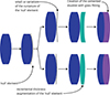 |
Figure 2 Saddle point construction example for the design of a doublet system. |
The SPC special version leads to several solutions with different numbers of surfaces where the variable a corresponds to the number of added elements. These solutions are then summed up in a tree diagram which enables the designer to select the most appropriate solution SP_a_p where p represents the number of the solution at depth a with p = [0, a2] (see Fig. 3).
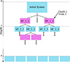 |
Figure 3 Tree diagram example for a saddle point construction of depth a, where a corresponds to the number of elements added to the system. The root system is a N elements optimized system, and the final system have (N + a) elements. |
The selected method enables the automatic generation of new starting points without prior knowledge. This method can be complementary to other AI methods by generating new datasets.
3. Design of achromatic cemented doublets with the SPC method
In the previous section, we explained the principle of the Saddle Point Construction method and its benefits. To validate the effectiveness of the method in optical design, we now apply it to the automatic design of an achromatic cemented doublet.
To evaluate the quality of the generated doublets, we compare them with achromatic doublets designed with a theoretical approach. The selected doublets for this comparison are drawn from [16], and from Thorlabs and Edmund Optics catalogues. Their common optical characteristics are tabulated in Table 1.
Characteristics of the selected doublets used for the comparison.
All selected doublets are made using Schott glasses as well as the designed doublets using the Saddle Point Construction Method.
In lens design, it is essential to consider the practical constraints in line with manufacturing capabilities [2]. The following constraints were imposed: a minimum center thickness, a minimum edge thickness, a minimum air gap, minimum and maximum curvatures (see values specified in Table 2 where SD is the semi-diameter of the lens). These constraints ensured the achromatic doublets designs remained manufacturable and mechanically robust.
Design constraints applied to the design of an achromatic doublet with the SPC method, where SD is the semi-diameter of the lens.
The designing process of the achromat is the following:
Start with a plane-parallel plate made of material Mj with a thickness of 4mm.
Optimize this initial configuration into a single lens with fixed focal length, F-number and with d the reference wavelength.
Apply the SPC method to this local minimum to generate two doublet systems integrating a fictitious glass.
Perform a glass substitution by fitting the fictitious glass to real materials, followed by a re-optimization of the optical system with the previous constraints.
The very last optimisation of the optical system is a local optimisation of transverse aberrations. The radii of curvature and the thickness of the lens elements are set as variables to minimise the spot diameter produced by the system.
The Figure 4 shows an example of a tree diagram with resulting RMS spot diameter at each step of the SPCM optimisation process. The initial system used as an example leads to the system 1 in the Table 4. The system 1 is represented by the bottom branch of the tree diagram with an RMS spot size of 0.004 mm.
 |
Figure 4 Example of RMS spot diameter evolution during the SPCM optimisation process, from initial system to final doublet after glass fitting. |
Configurations of the five best achromatic cemented doublets and their spot sizes in mm. R1, R2 and R3 are the radius of curvature of sequential surfaces in millimetres. tj are the center thickness of the two lenses in mm and s’ the back focal length of the achromatic cemented doublets in mm.
Schott glasses selected after principal component analysis of the Schott catalogue.
This routine is applied to the j materials of the Schott map, enabling to find 2 × j achromatic doublets.
To control the whole process, the Code V glass fitting algorithm was not used, but rather with a bespoke glass substitution Python algorithm. We then performed a search for the 10 closest real glasses to the fictitious glass. These 10 glasses minimise their distance to the fictitious glass as: (1)
(1)
where ΔGi is the Euclidean distance between the fictitious glass and the real glass i,  and
and  are the refractive indices of the fictious glass at the wavelength d, F, C, and
  ,
,  and
and  are the refractive indices of the real glass i at the wavelength d, F, C.
The fictitious glass is replaced by each of these 10 glasses one after the other. After a local optimization of the system, the glass leading to the smallest spot diagram is kept. This glass substitution process has been applied using the reduced glass map detailed in Section 4.
The Schott glass map from 2024 contains 120 glasses [17], which leads to the design of 240 doublets. Extending this method to N lenses needs the design of 120 × 2N optical system. For a Tessar lens, this would represent 1920 systems or 122 880 lenses for a 10 lenses objective. To minimize the computational effort, a reduction of the number of glasses is required.
4. Creation of a reduced glass map
Multiple attempts at reducing glass maps have been performed in recent decades [18–22]. This is possible since some glasses have very similar optical and chemical properties. The very first step of reducing the glass map would be to select only one glass from multiple glasses with similar optical properties. For instance, the Schott catalogue includes N-SF6, N-SF6HT, and N-SF6HTULTRA, three glasses with identical optical properties that differ mainly in their transmittance characteristics [23]. In such cases, retaining only one representative glass, typically the most cost-effective, can simplify the selection process. Applying this criterion to the full Schott glass map [17] and removing the lead containing and radiation resistant glasses, reduces the number of available glasses from 120 to 83. But the resulting set still remains too large for iterative procedures.
In the history of optical design, several dispersion models have been proposed to select glasses for the design of achromatic cemented doublets and apochromats [24–26]. Recently, H. Münz et al. [12] proposed a new graphical selection of glasses using principal component analysis (PCA) on the normalized index differences δj (λi):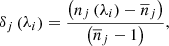 (2)
(2)
with nj (λi) the refractive index of the optical glass of the jth lens for the three wavelengths λC = 656,281 nm, λd = 587,562 nm, and λF = 486,134 nm and  the mean of the refractive indices across these three wavelengths.
This leads to two principal components, denoted δ(j, PC1) and δ(j, PC2). The principal component analysis, through the 83 optical glasses, transforms the basis of the δj diagram, resulting in δ(j, PC1) and δ(j, PC2) vectors which are combinations of the δj at different wavelengths and proportional to the 1st and 2nd order of colour aberrations respectively. These vectors are robust to changes in catalogues and wavelengths. The coefficients of the two principal components are normalized to a peak-to-valley deviation of 1 using the following equations: (3)
(3) (4)
(4)
The axial chromatic aberration for first and second order axial colour for a system of k thin lenses in contact can therefore be defined as: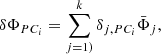 (5)
(5)
with  the partial refractive power of the lens j and
  the ith axial chromatic aberration. The resulting diagram for
  and
and  is shown in Figure 5, with
 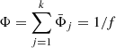 where f is the total focal length.
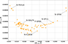 |
Figure 5 Diagram of the full Schott Glass map after principal component analysis. |
By tracing a straight line connecting two glasses and intersecting the  axis, i.e.
  , we can select a glass couple with first order axial colour corrected and
  . f as secondary axial colour. The ratio of the distances between the selected glasses and the resulting doublet on the diagram reflect the individual refractive power. A larger separation between the glasses implies lower required refractive powers for each element. Lower refractive powers allow for the use of lenses with larger radii of curvature, thereby reducing spherical aberrations. Therefore, to design a well-corrected achromatic doublet, it is better to select glasses that are widely separated in the diagram and connected by a line oriented toward, or as close as possible to, the origin.
Under the specified conditions some glasses cannot be combined with others to design an achromat. This provides a good basis on which to further reduce the glass catalogue. Because we are designing an achromat, it is not necessary to achieve  . Instead, glass combinations are selected to satisfy empirically
  values ranging from 0 to −3.5 × 10⁻⁴. This corresponds to a maximum allowable secondary axial colour of f/2857. A minimum separation of 0.012 was imposed between selected glasses on the map, to prevent the selection of materials with similar optical properties. Under these criteria, the glass map was reduced to a total of 34 glasses (see Fig. 6), tabulated in Table 3.
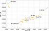 |
Figure 6 Diagram of the reduced Schott Glass map after principal component analysis and the application of empirically selected criteria (34 glasses). |
5. Results
5.1. Axial object field solutions on achromatic doublets
The SPC method, combined with the previous glass map, has led to the design of 68 achromatic doublets with a focal length of 100 mm and an f-number of 4. To assess the performance of achromatic cemented doublets, the spot sizes of the five best performing designed achromatic cemented doublets were compared with the five best achromatic cemented doublets designed by A. Szulc [16], as well as two off-the-shelf achromatic cemented doublets: Thorlabs reference AC254-100-A and Edmund Optics reference 47-641. As shown in Figure 7, the SPC method designed achromatic cemented doublets perform spot diameter approximately half the size of those produced by A. Szulc [16] and the off-the-shelf achromatic cemented doublets. The corresponding spot sizes and configurations are presented in Table 4, where Ri are the radius of curvature of sequential surfaces, tj are the center thickness of the two lenses and s’ the back focal length of the achromatic cemented doublets.
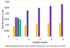 |
Figure 7 Spot size in mm produced by the achromatic cemented doublet designed by the SPC method (yellow), A. Szulc method (Purple) [16] and the two off-the-shelf achromatic cemented doublets from Thorlabs (green) and Edmund Optics (blue). |
To ensure the materials selected by the SPC method above are optimal, the diagram in Figure 6 was used to trace vectors connecting each pair of materials, allowing for the calculation of  and their separation. As shown in Table 5, all selected pairs satisfy the condition on
  . However, the minimum separation criterion was not met for two glass combinations: N-PK51 with N-LASF41, and N-PK52A with N-LASF41. But, the deviations for these two pairs are minimal, and the combinations do not involve glasses of the same type, suggesting that their inclusion remains acceptable within the context of the reduced glass map. Furthermore, these three glasses have been selected in the reduced glass map in combination with other glasses.
Glass combinations of the top 5 achromatic cemented doublets with  (at
(at  ) and their separations.
One of the resulting doublet examples is illustrated in Figure 8. This shows the total spot size of the best automatically generated doublet for the axial field, which has a diameter of 8.9 μm, as well as its MTF. The ray aberration diagram Figure 8d shows that for the green and blue wavelengths the curves almost overlap. We can therefore conclude that this generated system is almost diffraction-limited and colour corrected for the axial field.
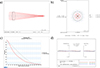 |
Figure 8 Results of achromat 1 designed with the Saddle Point Construction and a reduced glass map. (a) 2D Lens drawing of the system, (b) Spot Diagram of the system with Airy disk at reference wavelength displayed, (c) MTF of the system, (d) ray aberration curves. |
A Monte Carlo tolerance analysis was performed on the top-performing generated design and on the Thorlabs AC254-100-A achromatic cemented doublet. With typical manufacturing errors of ±0.05 mm and ±0.1° element tilt, it led to a maximum RMS Spot diameter of 0.8 for the generated achromatic cemented doublet and the Thorlabs AC254-100-A lens (see Fig. 9). This ensure equal performance of the two systems with the same manufacturing conditions.
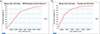 |
Figure 9 Results of a Monte Carlo Tolerance analysis with 50 cycles of (a) the top-performing achromatic cemented doublet and (b) the Thorlabs AC254-100-A lens. |
5.2. Non-axial object field solutions on achromatic doublets
When using achromatic doublets, it is impossible to achieve a 0° axial object field. They are most often used with a small field of view. To accurately compare our results with catalogue doublets we automatically generated cemented doublets for a field of view of ±2.5°.
Using the same method, 68 doublets were generated, and the one with the smallest spot size was selected for this comparison.
As shown in Figure 10, the SPCM can automatically generate achromatic cemented doublets with similar performances to catalogue doublets, with a field angle of 2.5°. These results were achieved by applying weights of 5 and 2 to field angles of 0° and 2.5° respectively. This produced a system with a comparable spot size for the axial object field and a spot size that is 14 μm smaller for the 2.5° angular object field. As shown Figure 11, the spot diameter progressively increases with the field of view without ensuring its performances across the field of view.
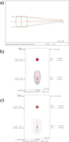 |
Figure 10 Example of an achromat designed with the Saddle Point Construction and a reduced glass map for an object field of 2.5° and spot size comparison with a Thorlabs achromatic cemented doublet. (a) 2D Lens drawing of the system. (b) Spot Diagram of the system with Airy disk at reference wavelength displayed. (c) Spot diagram of the Thorlabs AC254-100-A achromatic cemented doublet. |
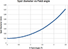 |
Figure 11 Spot diameter vs field of view of the generated lens Figure 10 a) with a total field of view of ±2.5°. |
By modifying the weight distribution across the field angles, we can minimise one field spot size at the expense of another. For example, setting the weights to 5 and 1 for field angles of respectively 0° and 2.5°, reduces the size of the central field spot, as well as the diameter of the 2.5° field spot (see Fig. 12). In addition, the resulting spot for blue and red wavelengths on the axial field are overlapping which is not the case for the doublet shown Figure 10. The overall performance of the two doublets, which were generated with a total FOV of ±2.5°,is comparable. However, diffraction has a stronger impact on the doublet optimised with weights of 5 and 1 for field angles of 0° and 2.5°. Despite having a smaller central spot diameter than the doublet optimised with weights of 5 and 2 for field angles of 0° and 2.5°, its MTF is farther from the diffraction limit (see Fig. 13).
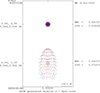 |
Figure 12 Spot size of an SPCM generated doublet optimized with weights of 5 and 1 for field angles of 0° and 2.5°. |
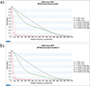 |
Figure 13 MTF of the doublets generated with the SPCM, (a) optimized with weights of 5 and 2 for field angles of 0° and 2.5°, (b) optimized with weights of 5 and 1 for field angles of 0° and 2.5°. |
The doublets designed using the SPCM and the selected doublet from Thorlabs show comparable axial chromatic aberrations (see Table 6). The doublet optimised with respective weights of 5 and 1 at 0° and 2.5° field of view, has a coma 10 times smaller than the first doublet designed with the SPCM and the selected Thorlabs doublet. The SPCM-designed doublets display spherical aberrations half the size of the Thorlabs doublet. However, their lateral chromatic aberration remains slightly stronger than that of the selected Thorlabs doublet.
Configurations of the two achromatic cemented doublets with non axial field generated with SPCM.
All simulations have been performed on a 13th Generation Intel® Core™ i7-1370P 3.90 GHz CPU computer with a 32 Go RAM using Python 3.11 and Code V 2024.03. The average computation time for the creation of the 34 solutions tree diagrams was about 24 minutes.
6. Conclusion
This article shows the effectiveness of the SPCM combined with a reduced glass map with automatic generation of lens systems. This has been demonstrated through the automatic design of 68 achromatic doublets. These designs respect manufacturing capabilities, with at least five configurations exhibiting superior optical performance for an axial field compared to existing solutions. The five best doublets, which were automatically generated using the SPCM, have a total spot size for an axial field with a diameter half that of the doublets selected in Section 3. When increasing the FOV to 5°, the doublets generated have similar performance as off-the-shelf doublets.
While glass cost was not considered in the present study, incorporating economic factors could provide an additional parameter for further reduction of the glass map. Moreover, the methodology could be extended to other or combined glass maps to expand the range of available materials. However, this approach currently only uses spherical and on-axis surfaces with a fixed stop aperture position. This is limiting the possibility of designing wide angle or very compact optical systems. By adding the possibility of using aspherical lenses could mitigate this limitation.
Finally, this approach may be generalized to the design of optical systems with a greater number of elements by applying SPCM at a deeper level in the solution tree. These systems could then be used as starting point for further optimisation with aspheres. Colour correction could also be extended to more wavelengths applying the Principal Component Analysis to additional wavelengths.
Funding
This work was funded by Optiive, under a contract with Satt/Conectus.
Conflicts of interest
Authors declares no conflict of interest associated to this work.
Data availability statement
Data underlying the results presented in this paper are not publicly available at this time but may be obtained from the authors upon reasonable request.
Author contribution statement
Investigation: H.G., P.T., R.P.;
Supervision: P.T., R.P., P.G., M.F.;
Methodology: H.M., P.T., R.P., P.G., M.F.;
Software: H.M., P.T., R.P.;
Validation: P.T., R.P., P.G., M.F.;
Visualization: H.M., P.T., R.P.;
Formal analysis: H.M., P.T., R.P., P.G., M.F.;
Funding acquisition: P.T., R.P., P.G., M.F.;
Writing – original draft: H.M.;
Writing – review & editing: P.T., R.P., P.G., M.F.
Acknowledgments
We acknowledge Optiive for its financial support of this work and A. Argy, F. Baumann, J. Belheine, P.-G. Bibal-Sobeaux and B. Brouillet for the first Python script on SPC method developed in IPP Team (ICube laboratory). We thank Paul Montgomery for carefully reading the manuscript.
References
- Bociort F, Optical System Optimization, in Encyclopedia of Optical and Photonic Engineering (Print) – Five Volume Set, 2nd edn., edited by C. Hoffman, R. Driggers (CRC Press, Boca Raton, 2015), pp. 2206–2212. https://www.taylorfrancis.com/books/9781351247184/chapters/10.1081/E-EOE2-120009685. [Google Scholar]
- Sun H, Lens design: a practical guide (CRC Press, Taylor & Francis Group, Boca Raton, 2017). [Google Scholar]
- Zhang K-Y, Yuan X-Y, Cui X-Q, Automatic generation of optical initial configuration based on Delano diagram, Res. Astron. Astrophys. 16(1), 007 (2016). https://iopscience.iop.org/article/10.1088/1674-4527/16/1/007. [Google Scholar]
- Côté G, Lalonde J-F, Thibault S, Deep learning-enabled framework for automatic lens design starting point generation, Opt. Exp. 29(3), 3841 (2021). https://opg.optica.org/abstract.cfm?URI=oe-29-3-3841. [Google Scholar]
- Yow AP, et al., Artificial intelligence in optical lens design, Artif. Intel. Rev. 57(8), 193 (2024). https://link.springer.com/10.1007/s10462-024-10842-y. [Google Scholar]
- Dai F, Feng H, Xu Z, Automatic design method for miniature aspheric lens based on modified basin-hopping algorithm, Opt. Exp 33(11), 22570 (2025). https://opg.optica.org/abstract.cfm?URI=oe-33-11-22570. [Google Scholar]
- Mao B, et al., FreeformNet: fast and automatic generation of multiple-solution freeform imaging systems enabled by deep learning. Photon. Res. 11(8), 1408 (2023). https://opg.optica.org/abstract.cfm?URI=prj-11-8-1408. [Google Scholar]
- Bociort F, Finding new local minima in lens design landscapes by constructing saddle points, Opt. Eng. 48(6), 063001 (2009). http://opticalengineering.spiedigitallibrary.org/article.aspx?doi=10.1117/1.3156022. [Google Scholar]
- Livshits I, et al., Using saddle points for challenging optical design tasks, in SPIE Proceedings, edited by RB Johnson, VN Mahajan, S Thibault (San Diego, California, United States, 2014), p. 919204. http://proceedings.spiedigitallibrary.org/proceeding.aspx?doi=10.1117/12.2061975 [Google Scholar]
- Van Grol P, Van Turnhout M, Bociort F, Obtaining different lens system shapes by using Saddle-Point Construction, in Classical Optics 2014 (Kohala Coast, Hawaii, 2014), p. IW1A.3. https://opg.optica.org/abstract.cfm?URI=IODC-2014-IW1A.3. [Google Scholar]
- Van Turnhout M, et al., Obtaining new local minima in lens design by constructing saddle points. Opt. Exp. 23(5), 6679 (2015). https://opg.optica.org/abstract.cfm?URI=oe-23-5-6679. [Google Scholar]
- Münz H, Peschka M, Principal component analysis of refractive index spaces: From glass properties to residual colour prediction. EPJ Web Conf. 309, 03019 (2024). https://www.epj-conferences.org/10.1051/epjconf/202430903019. [Google Scholar]
- Hou Z, Systematic search for new solutions in lens design. Disertation. Delft University of Technology, 2023https://doi.org/10.4233/uuid:485031ef-4fcf-4c2f-9a6b-41b037e88afe. [Google Scholar]
- Marinescu O, Bociort F, Network search method in the design of extreme ultraviolet lithographic objectives. Appl. Opt. 46(35), 8385 (2007). https://opg.optica.org/abstract.cfm?URI=ao-46-35-8385. [Google Scholar]
- Bociort F, Van Turnhout M., Marinescu O, Practical guide to saddle-point construction in lens design, in SPIE Proceedings, edited by PZ Mouroulis, WJ Smith, RB Johnson (San Diego, CA, 2007), p. 666708. [Google Scholar]
- Szulc A, Improved solution for the cemented doublet, Appl. Opt. 35(19), 3548 (1996). https://opg.optica.org/abstract.cfm?URI=ao-35-19-3548. [Google Scholar]
- Schott AG, Schott optical glass datasheet collection (2024). [Google Scholar]
- Zhang S, Shannon RR, Lens design using a minimum number of glasses, in SPIE Proceedings, vol. 2263, edited by RE Fischer, WJ Smith (San Diego, CA, 1994), pp. 2–9. [Google Scholar]
- Besenmatter W, How many glass types does a lens designer really need? in International Optical Design Conference, Kona, HI, edited by LR Gardner, KP Thompson (1998), p. 294. [Google Scholar]
- Griffin DW, Selection of optical glasses using Buchdahl’s chromatic coordinate, in International Optical Design Conference, Kailua-Kona, Hawaii (1998), p. LTuC.7. https://opg.optica.org/abstract.cfm?URI=IODC-1998-LTuC.7. [Google Scholar]
- Sola La Serna P., Sánchez-Capuchino Revuelta J. Optical glass selection for color corrected broadband instrumentation: an overview, Appl. Opt. 61(3), A50 (2022). https://opg.optica.org/abstract.cfm?URI=ao-61-3-A50. [Google Scholar]
- Héron S, Semet Y, Visible imaging system optical design by continuous optimization of glasses, EPJ Web Conf. 287, 02009 (2023). https://www.epj-conferences.org/10.1051/epjconf/202328702009. [Google Scholar]
- Schott AG, HT and HTultra Glass Optical glasses with ultra high transmittance (2025). [Google Scholar]
- Lytle JD, Design of apochromats by graphical construction, in SPIE Proceedings, edited by WJ Smith (San Diego, 1974), pp. 239–246. [Google Scholar]
- Robb PN, Selection of optical glasses 1: Two materials, Appl. Opt. 24(12), 1864 (1985). https://opg.optica.org/abstract.cfm?URI=ao-24-12-1864. [Google Scholar]
- Münz H, Sacks JA, Bentley JL, Single-term theory of induced secondary axial color. Opt. Eng. 64(3), 035101 (2025). https://www.spiedigitallibrary.org/journals/optical-engineering/volume-64/issue-03/035101/Single-term-theory-of-induced-secondary-axial-color/10.1117/1.OE.64.3.035101.full. [Google Scholar]
All Tables
Design constraints applied to the design of an achromatic doublet with the SPC method, where SD is the semi-diameter of the lens.
Configurations of the five best achromatic cemented doublets and their spot sizes in mm. R1, R2 and R3 are the radius of curvature of sequential surfaces in millimetres. tj are the center thickness of the two lenses in mm and s’ the back focal length of the achromatic cemented doublets in mm.
Schott glasses selected after principal component analysis of the Schott catalogue.
Glass combinations of the top 5 achromatic cemented doublets with (at ) and their separations.
Configurations of the two achromatic cemented doublets with non axial field generated with SPCM.
All Figures
|
Figure 1 Example of a saddle point generated by the augmentation of dimensionality of the optimisation landscape from a 1D merit function (left) to a 2D merit function (right). |
| In the text | |
|
Figure 2 Saddle point construction example for the design of a doublet system. |
| In the text | |
|
Figure 3 Tree diagram example for a saddle point construction of depth a, where a corresponds to the number of elements added to the system. The root system is a N elements optimized system, and the final system have (N + a) elements. |
| In the text | |
|
Figure 4 Example of RMS spot diameter evolution during the SPCM optimisation process, from initial system to final doublet after glass fitting. |
| In the text | |
|
Figure 5 Diagram of the full Schott Glass map after principal component analysis. |
| In the text | |
|
Figure 6 Diagram of the reduced Schott Glass map after principal component analysis and the application of empirically selected criteria (34 glasses). |
| In the text | |
|
Figure 7 Spot size in mm produced by the achromatic cemented doublet designed by the SPC method (yellow), A. Szulc method (Purple) [16] and the two off-the-shelf achromatic cemented doublets from Thorlabs (green) and Edmund Optics (blue). |
| In the text | |
|
Figure 8 Results of achromat 1 designed with the Saddle Point Construction and a reduced glass map. (a) 2D Lens drawing of the system, (b) Spot Diagram of the system with Airy disk at reference wavelength displayed, (c) MTF of the system, (d) ray aberration curves. |
| In the text | |
|
Figure 9 Results of a Monte Carlo Tolerance analysis with 50 cycles of (a) the top-performing achromatic cemented doublet and (b) the Thorlabs AC254-100-A lens. |
| In the text | |
|
Figure 10 Example of an achromat designed with the Saddle Point Construction and a reduced glass map for an object field of 2.5° and spot size comparison with a Thorlabs achromatic cemented doublet. (a) 2D Lens drawing of the system. (b) Spot Diagram of the system with Airy disk at reference wavelength displayed. (c) Spot diagram of the Thorlabs AC254-100-A achromatic cemented doublet. |
| In the text | |
|
Figure 11 Spot diameter vs field of view of the generated lens Figure 10 a) with a total field of view of ±2.5°. |
| In the text | |
|
Figure 12 Spot size of an SPCM generated doublet optimized with weights of 5 and 1 for field angles of 0° and 2.5°. |
| In the text | |
|
Figure 13 MTF of the doublets generated with the SPCM, (a) optimized with weights of 5 and 2 for field angles of 0° and 2.5°, (b) optimized with weights of 5 and 1 for field angles of 0° and 2.5°. |
| In the text | |
Current usage metrics show cumulative count of Article Views (full-text article views including HTML views, PDF and ePub downloads, according to the available data) and Abstracts Views on Vision4Press platform.
Data correspond to usage on the plateform after 2015. The current usage metrics is available 48-96 hours after online publication and is updated daily on week days.
Initial download of the metrics may take a while.