| Issue |
J. Eur. Opt. Society-Rapid Publ.
Volume 22, Number 1, 2026
|
|
|---|---|---|
| Article Number | 25 | |
| Number of page(s) | 10 | |
| DOI | https://doi.org/10.1051/jeos/2026014 | |
| Published online | 17 April 2026 | |
Research Article
Laplace–Beltrami shape analysis of ocular or wavefront surfaces
Instituto de Óptica (CSIC), Serrano 121, Madrid, Spain
* Corresponding author: This email address is being protected from spambots. You need JavaScript enabled to view it.
Received:
2
December
2025
Accepted:
8
February
2026
Abstract
Shape analysis techniques are widely used across biomedical fields for processing surface shape properties. The Laplace–Beltrami operator, as an extension of the Laplacian to surfaces, reveals geometrical properties related to surface curvature through its spectral decomposition, making it a promising tool in visual optics. I introduce Laplace–Beltrami shape analysis for ocular, or wavefront, surfaces of the human eye, described as meshes. I present a set of techniques and their numerical implementation for this purpose. Two particular tools, spectral decomposition and shape-DNA analysis, are explained in detail and illustrated with an example of application: a keratoconus cornea model.
Key words: Laplace–Beltrami operator / Shape analysis / Ocular surfaces / Surface curvature
© The Author(s), published by EDP Sciences, 2026
 This is an Open Access article distributed under the terms of the Creative Commons Attribution License (https://creativecommons.org/licenses/by/4.0), which permits unrestricted use, distribution, and reproduction in any medium, provided the original work is properly cited.
1 Introduction
The progress in high-resolution and efficient optical metrology technologies –such as optical coherence tomography or intensity-based wavefront sensing [1–3] – applied to measuring either ocular interfaces or, indirectly, the wavefront surface has permeated ophthalmology practice. The highly dense sampling of these surfaces consequently leads, at least for some applications, to local surface representations such as splines [4, 5] or mesh surfaces [6], i.e., those constructed by a set of polygonal faces, typically triangles. Furthermore, these high-spatial-sampled surfaces encourage the application of spectral analysis to them. For instance, classical Fourier techniques have been proposed for analysing keratoconus eyes – i.e. an eye condition characterized by a thinning and bulging of the cornea degrading vision – through wavefront phase imaging [3]. Besides Fourier analysis, Zernike decomposition of optical surfaces is undoubtedly the most typical approach to analyze, or characterize, optical wavefront or surfaces. However, both Zernike and Fourier coefficients do not fully capture the shape information, especially the effect of curvature on the spectrum itself [7]. Indeed, this intrinsic limitation of conventional Zernike polynomials led to the proposal of some alternatives, such as the so-called Zernike curvature polynomials [8]. However, these are only valid when the surface gradient is small, so the wavefront curvature reduces to its Laplacian; an approximation that is not sustained in many practical cases.
By analogy to classical Fourier analysis, spectral methods over surfaces defined as meshes were introduced at the end of the last century for discrete geometry processing [7]. The goal of these methods is to capture the geometrical shape properties of the surface, which is referred to as shape analysis. Mesh surfaces are especially suitable for shape analysis thanks to the fact that discrete differential geometry techniques can be directly applied to them [9]. A pioneering work in spectral methods over meshes was that of Taubin [10], which defined the mesh vertex coordinates as a 3D signal and applied Laplacian operators. Another option is to define a scalar function over the mesh surface.
Surface spectral methods comprise three steps: 1) selecting an appropriate linear operator; 2) the eigendecomposition of that operator; and 3) employing the spectral eigenvalues and eigenvectors in a specific manner according to the processing purpose. In other words, spectral methods inspect a surface by examining the eigenvalue decomposition of a meaningful selected linear operator. Therefore, the application at hand determines the selection of the linear operator and how to employ the spectrum.
Surface spectral methods have been used intensively in a diversity of techniques [11], such as mesh compression [12, 13], segmentation [14], smoothing or denoising through filtering [15], symmetry detection [16, 17], surface reconstruction from point clouds [18], or watermarking [19], all of them relevant in image processing applications.
As mentioned before, the first and most crucial step in spectral methods is the selection of an appropriate linear operator. In optics, the curvature – in its various mathematical forms – is the most relevant geometrical property because it linearly depends on the optical power, the fundamental property in all imaging systems. In any form, the curvature involves second-order derivatives, so a mandatory choice for such an operator is that it should include them. Then, the Laplace–Beltrami operator emerges as the best option because it involves second-order derivatives, but it is linear within the surface geometry coordinates. Here, I use the so-called geometric mesh Laplacian, because it explicitly encodes the geometric information of the mesh [7]. Furthermore, selecting a curvature-based local shape index as the scalar function defined over the mesh leads to an optically meaningful Laplace–Beltrami spectrum [7, 20]. One of the potentials of the Laplace–Beltrami, for our purposes, stems from the fact that it characterizes the smoothness of a scalar function over a surface, grosso modo, the difference between the scalar at a point P and a weighted average in a small neighborhood of P (Sect. 6.2 [7]).
For certain applications, shape analysis focuses on capturing morphologically relevant shape descriptors, also called signatures or fingerprints. Such a signature has been called shape-DNA; so, from now on, I will follow this notation [11]. As it will be seen, employing a local curvature shape index scalar (for instance, the Gaussian curvature) notably increases the discrimination capacities of the Laplace–Beltrami spectrum.
To date, I am not aware that geometric mesh analysis has been applied in the visual optics literature, except for a paper in retina imaging [21]. I believe that there is a call to introduce these techniques, especially for analysing anterior chamber depth interfaces, ocular wavefront surfaces, or even ophthalmic lens surfaces. In this paper, I present a systematic approach to these techniques and provide some applications. A major hypothesis is that surface second-order differential features, captured by the Laplace–Beltrami spectrum, can be employed to detect, compare, and study ocular surface shape features. The paper is organized as follows. First, in Section 2, I introduce all the basic mathematical aspects of the Laplace–Beltrami spectra decomposition theory. Next, in Section 3, I introduce a particular, but meaningful, geometric eye surface-thickness model that will be used in subsequent sections, particularly a keratoconus model. Subsequently, in Sections 4 and 5, I present two relevant applications of the theory: the spectral decomposition and the shape-DNA analysis, respectively. Finally, in Section 6, I summarize results and discuss their implications.
2 Laplace–Beltrami spectral decomposition theory
The Laplacian operator (Δ), i.e., the divergence of the gradient  , measures how a function differs from its average in a local neighborhood. The Laplace–Beltrami operator is a generalization of the Laplacian to functions defined over surfaces or manifolds in higher dimensions.
Let f ∈ C
2 be a real-valued function (continuous second derivatives) defined over a smooth bounded surface S, locally represented by a parametrization: r(x, y) ≡ (x, y, z(x, y)): S
2 → R
3, being S
2 a two-dimensional (circular or not) Cartesian parametric domain. Denoting  and
and  , the Riemannian metric tensor or first fundamental form matrix (symmetric) is:
![Mathematical equation: $$ \left[\begin{array}{cc}{g}_{11}& {g}_{12}\\ {g}_{21}& {g}_{22}\end{array}\right]\equiv \left[\begin{array}{cc}{\mathbf{r}}_x{\mathbf{r}}_x& {\mathbf{r}}_x{\mathbf{r}}_y\\ {\mathbf{r}}_y{\mathbf{r}}_x& {\mathbf{r}}_y{\mathbf{r}}_y\end{array}\right]=\left[\begin{array}{cc}(1+{z}_x{)}^2& {z}_x{z}_y\\ {z}_x{z}_y& (1+{z}_y{)}^2\end{array}\right], $$](/articles/jeos/full_html/2026/01/jeos20250090/jeos20250090-eq4.gif)
which determinant is  .
.
Now, fx, fy, fxx, fyy, fxy, denoting partial derivatives of f and considering relations between the elements of the Riemannian metric and those of the inverse matrix (p. 153 [22]), the Laplace–Beltrami operator over f is defined as [23]:![Mathematical equation: $$ {\Delta }_g[f]=\frac{{g}_{12}\left({f}_{{yx}}-{\mathrm{\Gamma }}_{21}^1{f}_x-{\mathrm{\Gamma }}_{21}^2{f}_y\right)-{g}_{11}\left({f}_{{yy}}-{\mathrm{\Gamma }}_{22}^1{f}_x-{\mathrm{\Gamma }}_{22}^2{f}_y\right)}{g}-\frac{{g}_{22}\left({f}_{{xx}}-{\mathrm{\Gamma }}_{11}^1{f}_x-{\mathrm{\Gamma }}_{11}^2{f}_y\right)-{g}_{12}\left({f}_{{xy}}-{\mathrm{\Gamma }}_{12}^1{f}_x-{\mathrm{\Gamma }}_{12}^2{f}_y\right)}{g}. $$](/articles/jeos/full_html/2026/01/jeos20250090/jeos20250090-eq7.gif) (1)
(1)
Here,  are the so-called Christoffel symbols; their values as a function of partial derivatives of z have been derived elsewhere [24]:
I note that the Laplace–Beltrami operator encodes the intrinsic geometry, i.e., that part of it not depending on the surface parameterization, so any other parametrization (e.g., polar parametrization) instead of the Cartesian one would provide the same geometrical structure. Also, it is worth mentioning that when the local curvature of the surface is quasi-flat (zx, zy ≪ 1), the Laplace–Beltrami operator is approximately equal to the Laplacian.
In discretized surfaces, the discrete Laplace operator replaces the continuous one. The surface is described by a triangular mesh M, described by a set of geometric vertices coordinates, a matrix V = (x1, …, xn, y1, …, yn, z1, ..., zn), and an ordering collection of those vertices through edges. Then, the discrete Laplace–Beltrami operator (ΔM) of a scalar function f at a vertex i can be estimated with the cotangent formula [7]:![Mathematical equation: $$ {\Delta }_M[f{]}_i=\frac{1}{2{A}_i}\sum_j (\mathrm{cot}\enspace {\alpha }_{{ij}}+\mathrm{cot}\enspace {\beta }_{{ij}})({f}_j-{f}_i), $$](/articles/jeos/full_html/2026/01/jeos20250090/jeos20250090-eq12.gif) (2)where the sum is over all adjacent vertices j of i, αij and βij are the two angles subtended by the edge joining i and j, and Ai is the vertex area of i.
(2)where the sum is over all adjacent vertices j of i, αij and βij are the two angles subtended by the edge joining i and j, and Ai is the vertex area of i.
The computation of equation (2) is facilitated if the operator is encoded in matrix form that is obtained by the product of a diagonal matrix and a symmetric matrix (Sect. 6.2 [7]): (3)where
  is the diagonal matrix whose entries are 1/2Ai and
  is a symmetric matrix – the so-called cotangent – encoding the sum of the cotangent angles. The Laplacian matrix is largely sparse, with an average of seven non-zero values per row [7]. However, the matrix
  is, in general, not symmetric, which makes the eigenvalue problem more demanding. Luckily,
  is symmetric, so a good approach (followed here) is to obtain the spectral decomposition by solving the generalized eigenvalue problem (Sect. 9.1 [7]):
 (4)which provides the same spectral decomposition as finding the eigenvalues of
  directly.
I solved the generalized eigenvalue problem of equation (4) using Matlab(R) built-in function eigs.m.
The eigenvectors obtained are sorted in ascending eigenvalues: ![Mathematical equation: $ \mathcal{T}=[{\phi }_1,...,{\phi }_k]$](/articles/jeos/full_html/2026/01/jeos20250090/jeos20250090-eq20.gif) , and excluding the smallest eigenvalue ϕ0 that is zero, so such a truncated decomposition can be interpreted as a low-pass filter because the smallest eigenvalues correspond to the less ‘curved’ eigenvectors.
, and excluding the smallest eigenvalue ϕ0 that is zero, so such a truncated decomposition can be interpreted as a low-pass filter because the smallest eigenvalues correspond to the less ‘curved’ eigenvectors.
Then, the Laplace–Beltrami spectral reconstruction of the surface mesh is obtained by applying the matrix transformation [25]: (5)where, recall, that
  is the mesh vertex matrix.
2.1 Laplace–Beltrami spectra of scalar functions defined over the mesh
Given the scalar function f defined over the mesh M, the set of Laplace–Beltrami eigenfunctions makes it possible to perform a spectral decomposition of f on S, provided that the eigenfunctions are normalized such that (ϕi
, ϕj) = δi,j. We denote this set of normalized eigenvectors: ![Mathematical equation: $ {T}_n=[{\phi }_{n1},...,{\phi }_{{nk}}]$](/articles/jeos/full_html/2026/01/jeos20250090/jeos20250090-eq23.gif) . Then, the Laplace–Beltrami spectrum is obtained by a projective matrix operation [7]:
. Then, the Laplace–Beltrami spectrum is obtained by a projective matrix operation [7]: (6)
(6)
As will be presented later, I have evaluated the Laplace–Beltrami spectra of two scalar functions: thickness and Gaussian curvature, and for a specific simulation the mean curvature.
Evaluating the Gaussian curvature (or any other differential quantity on the mesh) involves a trade-off in the neighbourhood size used for numerical estimations. Although for data free of noise, smaller sizes increase accuracy, in the presence of noise, larger neighbourhoods may be more robust to the effect of noise. In Section 3, this trade-off will be illustrated.
For Gaussian curvature computation, the first step is to estimate a normal vector ni associated with each vertex of the mesh surface. This was done by taking the weighted average of the normals associated with each face touching the vertex [26]. The weights were chosen by following the procedure proposed at [27]. Then, selecting a direction determined by two, pi and pj, neighbourhood vertices points, the normal curvature at pi in that direction is given by [26]: (7)
(7)
Now, similar to how the first fundamental form is defined, the second fundamental form, denoting n the surface normal, is:![Mathematical equation: $$ \left[\begin{array}{cc}{b}_{11}& {b}_{12}\\ {b}_{21}& {b}_{22}\end{array}\right]\equiv \left[\begin{array}{cc}{\mathbf{r}}_{{xx}}\mathbf{n}& {\mathbf{r}}_{{xy}}\mathbf{n}\\ {\mathbf{r}}_{{yx}}\mathbf{n}& {\mathbf{r}}_{{yy}}\mathbf{n}\end{array}\right]=\left[\begin{array}{cc}\frac{{z}_{{xx}}}{\sqrt{1+{z}_x^2+{z}_y^2}}& \frac{{z}_{{xy}}}{\sqrt{1+{z}_x^2+{z}_y^2}}\\ \frac{{z}_{{yx}}}{\sqrt{1+{z}_x^2+{z}_y^2}}& \frac{{z}_{{yy}}}{\sqrt{1+{z}_x^2+{z}_y^2}}\end{array}\right]. $$](/articles/jeos/full_html/2026/01/jeos20250090/jeos20250090-eq26.gif)
From the set of normal and normal curvatures, an estimation of the second fundamental matrix above is obtained using least squares [28]. Finally, I recall that the principal curvatures, k1 and k2, are the eigenvalues of the second fundamental form, the Gaussian curvature is its product:  , and the mean curvature its average
  . In practice, for curvature computations, I used Matlab code developed by Itzik Ben, freely available at: https://es.mathworks.com/matlabcentral/fileexchange/47134-curvature-estimationl-on-triangle-mesh.
3 Example of application: artificial eye surface model
On the one hand, anterior segment ocular surface interfaces (crystalline lenses and cornea) can be modelled to some extent as a biconic function [29] plus some perturbation terms. On the other hand, a certain type of surface perturbation can be generically described with a Gaussian function; for instance, a keratoconus [30]. Considering the above, as an example of application, I modelled an anterior cornea surface topography at each (x, y) location with the following equation: (8)and the thickness at each point with:
 (9)
(9)
The piston term is just an arbitrary number – particularly, 10 – selected to avoid negative numbers in z, but, of course, without changing the shape. Following equation (8), I computed the Gaussian curvature following the procedure described in Section. 2.1. These functions are defined within a circular domain  . Considering that real biometric data is affected by measurement noise, I added white Gaussian noise to the z values with the Matlab function awgn. The level of Gaussian noise was simulated through the Signal-to-Noise Ratio (SNR), whose units are dBs.
Figure 1 plots the surface mesh, the Gaussian curvature, and the thickness corresponding to these equations with the following parameters: Rx = 7.79 mm, Ry = 7.61 mm, Qx = −0.27, Qy = −0.27, h0 = 0.2 mm, σx = 0.5, σy = 0.5, x0 = 1.5 mm, and y0 = −1.5 mm and with a SNR = 90 dB. From now on, this cornea model will be referred to as test A.
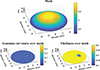 |
Figure 1 Mesh, Gaussian curvature, and thickness (mm) over the mesh of reference cornea A. |
As mentioned in Section 2.1, there is a trade-off between mesh density and noise level. To exemplify this fact, I computed the Gaussian curvature map for two noise levels: low noise (SNR = 90 dB) and moderate noise (SNR = 70 dB), and three levels of mesh sampling density determined by the number of mesh vertices: 5.025, 20.081, and 45.225 points. Figure 2 shows the results. Although for low noise, the more accurate Gaussian curvature estimation is achieved with high sampling density (45.225 mesh points), for moderate noise, the best estimation requires fewer mesh sampling points (between 20.081 and 45.225). Therefore, the choice a priori of the optimal mesh density, to improve the SNR ratio, is not an easy task because it also depends on the geometry shape. Nevertheless, a rule of thumb is that the stronger the local curvature changes, the denser the mesh required.
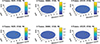 |
Figure 2 Gaussian curvature over mesh of surface test A for different mesh densities and two levels of noise: SNR = 70 dB and SNR = 90 dB. |
4 Spectral decomposition
A first potential of the Laplace–Beltrami operator comes from its spectral decomposition obtained with equation (5). As mentioned in the introduction, it can be used for mesh compression or smoothing through filtering. In both cases, the Laplace–Beltrami operator serves to separate the curvature shape features of the surface in question. The first eigenvectors of the spectral decomposition (associated with low eigenvalues) capture the low-curvature shape signal, whereas the following ones apprehend the high-curvature part of the shape.
Figure 3 shows the mesh reconstruction of surface test A with an SNR = 80 dB for different numbers of eigenvectors in the spectral decomposition, particularly: 5, 10, 25, 50, 75, 100, 200, and 300. The figure shows that only when more than approximately 50 eigenvectors are included does the “bump” part of the keratoconus start to be revealed. Note that, as with any spectral method, some artifacts are introduced at the periphery. This problem, related to the boundary conditions in the Laplace–Beltrami will be discussed in Section 6.
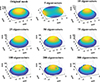 |
Figure 3 Original mesh corresponding to surface model A and spectral mesh reconstruction using different numbers of eigenvectors in the spectral decomposition. |
Generally, the problem of choosing the optimal number of eigenvectors would depend on the shape structure and the level of measurement noise. Therefore, preliminary modelling of the shape features of interest would surely help in that selection.
5 Laplace–Beltrami for shape-DNA analysis of ocular surfaces
A substantial benefit of the Laplace–Beltrami spectra is their invariance to isometric changes. These are deformations that preserve the length of every arc on the surface, so they conserve the shape. The most common isometric changes are rigid motions (rotation or global translation) and similarity scaling [11]. On the one hand, rotation or global translation is a typical issue due to eye fixation changes among measurements, for instance, in optical coherence tomography [31]. On the other hand, different eyes may differ in size but not in ocular shape; in this case, the Laplace–Beltrami spectra would be simply scaled, as will be shown.
The isometric invariance of the Laplace–Beltrami spectrum enables its use to extract geometrical fingerprints characterizing ocular surfaces, which has been coined a shape-DNA [11]. This signature is derived from the Laplace–Beltrami spectra as computed through equation (6).
The shape-DNA emerges akin to Fourier analysis as a spectral tool analysis, but contrary to the latter, a tool that captures better the shape geometry. Also, contrary to Fourier analysis, the surface mesh geometry determines different eigenbases of the Laplace–Beltrami spectrum, so the corresponding eigenvalues of different meshes cannot be directly compared; some type of normalization is required so that the shape-DNA is invariant to the surface’s size [7, 11]. Particularly, I propose scaling the Laplace–Beltrami spectra coefficients to the first coefficient:  , a procedure that is appropriate when trying to identify a surface shape pattern [11].
Furthermore, to apply the shape-DNA for quantitative comparison purposes, or to identify surface-mesh shape patterns, a distance metric must be constructed [11]. Given two arbitrary shape-DNAs (normalized set of eigenvalues): λ = (λ1, λ2, … λn) and μ = (μ1, μ2, … μn), from now on it will be used the 2-norm distance, which is unitless because the above normalization, expressed as: (10)
(10)
5.1 Shape-DNA similarity: continuous deformation
The shape-DNA offers a way to quantitatively track, with a single metric, the timing of ocular surface shape changes. This could be useful, for instance, as a clinical tool to analyze the time evolution of pathologies manifested by surface shape abnormalities. The underlying mathematical principle is that of similarity; namely, the shape-DNA fingerprint should depend continuously on shape deformations [11].
As an example, I propose an artificial model of keratoconus variation more or less compatible with the reported literature [32]. Starting with surface model A, I modelled a surface elevation change and thinning of the cornea with time manifested by a change of ho ranging from 0.2 to 0.4; and, synchronous with this process, a spatial expansion of the local abnormality modelled by a change of σx and σy values from 0.5 to 2. Three different shape-DNA were generated: associated with the Gaussian curvature, the mean curvature, and with the cornea thickness.
I computed the shape-DNA distance (Eq. (10)) between all these values and the initial reference value (ho = 0.2, σx = 1, and σy = 1), sampling the ranges in 100 steps. Results are plotted in Figure 4, revealing that the similarity principle is fulfilled, because the shape-DNA fingerprint depends smoothly on the continuous variation of the ho,σx and σy. However, it should be observed that this dependence is not necessarily linear or even monotonically increasing, as revealed by the Gaussian and mean curvature curvature fitting curves. Also, the relation depends strongly on the scalar function defined over the mesh, as revealed by the difference in the fitting curves of the Gaussian curvature and thickness. To complement this figure, Figure 5 shows the mesh, Gaussian curvature, and thickness for three representative stages of the previous timing model.
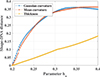 |
Figure 4 Shape-DNA distance to reference cornea model A for different scalar functions – Gaussian curvature, mean curvature and thickness – as function of timing surface deformation: explicitly the ho parameter, but implicitly also σx and σx. |
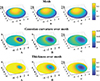 |
Figure 5 Surface meshes and Gaussian curvature as function of shape timing deformation: A) ho = 0.264, σx = 0.98, and σy = 0.98; B) ho = 0.332, σx = 1.49, and σy = 1.49; C) ho = 0.4, σx = 2, and σy = 2. |
5.2 Shape-DNA similarity: stability
As mentioned before, the isometry invariance of the Laplace–Beltrami operator implies that the fingerprint should not differ between surfaces that can be isometrically mapped onto each other. The most common isometrical mappings are rigid motions and scalings. Additionally, as it will be shown in Figure 6, the Gaussian curvature has the same value at corresponding points of isometric surfaces (p. 177 [33]).
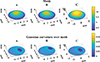 |
Figure 6 Surface, Gaussian curvature and thickness over meshes: A) Reference mesh; B) Reference mesh transformed by an eye fixation change. C) Reference mesh transformed through a uniform scaling. |
Starting again with reference surface A, I generated two isometric surfaces to it, exemplifying two typical scenarios found in visual optics biometry. In the first case, I modelled a change in eye fixation between two measurements of the same ocular surface as a direct rigid transformation between points of the original mesh [xi, yi, zi] onto the transformed one [xf, yf, zf] based on the matrix operator given by the equation:![Mathematical equation: $$ \left[\begin{array}{l}{x}_i\\ {y}_i\\ {z}_i\\ 1\end{array}\right]=\left[\begin{array}{llll}{R}_{11}& {R}_{12}& {R}_{13}& {t}_x\\ {R}_{21}& {R}_{22}& {R}_{23}& {t}_y\\ {R}_{31}& {R}_{32}& {R}_{33}& {t}_z\\ 0& 0& 0& 1\\ & & & \end{array}\right]\times \left[\begin{array}{l}{x}_f\\ {y}_f\\ {z}_f\\ 1\end{array}\right], $$](/articles/jeos/full_html/2026/01/jeos20250090/jeos20250090-eq36.gif) (11)where tx, ty and tz are translations along directions x, y and z; and Rij are entries of the Euler rotation matrix [34]. I implemented this with the help of the Matlab function rigidtform3d.m. Particularly, I modelled an eye fixation change provided by an Euler angle α = 45° and a translation defined by [tx, ty, tz] = [0.4, 0, 0]. Applying this transformation to the reference surface A, surface B is obtained.
(11)where tx, ty and tz are translations along directions x, y and z; and Rij are entries of the Euler rotation matrix [34]. I implemented this with the help of the Matlab function rigidtform3d.m. Particularly, I modelled an eye fixation change provided by an Euler angle α = 45° and a translation defined by [tx, ty, tz] = [0.4, 0, 0]. Applying this transformation to the reference surface A, surface B is obtained.
In a second example, I modelled a uniform scaling transformation that isotropically enlarges or shrinks the ocular surface by a scale factor equally in all directions. This is implemented through a scaling matrix operator.![Mathematical equation: $$ \left[\begin{array}{l}{x}_i\\ {y}_i\\ {z}_i\end{array}\right]=\left[\begin{array}{lll}\upsilon & 0& 0\\ 0& \upsilon & 0\\ 0& 0& \upsilon \\ & & \end{array}\right]\times \left[\begin{array}{l}{x}_f\\ {y}_f\\ {z}_f\end{array}\right], $$](/articles/jeos/full_html/2026/01/jeos20250090/jeos20250090-eq37.gif) (12)where υ is the scalar factor. Using a scaling dilatation υ = 1.005 onto the surface A, generate surface C.
(12)where υ is the scalar factor. Using a scaling dilatation υ = 1.005 onto the surface A, generate surface C.
The meshes and Gaussian curvatures over them of surfaces A, B, and C are depicted in Figure 6. It illustrates the change in eye fixation between surface B and A, as well as the uniform dilatation of mesh C with respect to A. Observing the Gaussian curvature map, its invariance with scaling shows the potential of this map with respect to plain meshes.
The shape-DNA distances between reference surface A, and surfaces B, C, are 8E–13, and 3E–13, respectively; quantities which are clearly negligible.
6 Conclusion
The large increase, in recent times, of the biometry capabilities applied to the anterior segment of the eye has led to a synchronous development of data processing techniques, which include compact and statistical surface representation [35, 36], image segmentation [37], or data interpolation/extrapolation [38, 39]. A similar process has occurred in reconstructing, modelling, or analyzing wavefronts [3, 40].
However, all these techniques, although indirectly dealing with curved surfaces, do not fully address the curvature shape information. In this sense, the Laplace–Beltrami spectral decomposition may emerge as a new tool offering this advantage. Of course, further exploration of the potential of the methodologies proposed in this paper requires testing them with real clinical data, such as optical coherence tomography measurements or highly dense wavefront sensor data.
As shown, the spectra are especially suitable for performing shape analysis through shape-DNA fingerprints. However, these fingerprints can be spatially localized, occupying different scales. When the objective is to perform a global shape comparison, but at the same time compare local geometrical features, a possible approach is to pick up the spectra associated with selected eigenfunctions [20]; for instance, in the discriminative representation of brain morphology [41]. This is something that could be explored in the future.
In the mathematical part, Laplace–Beltrami spectral theory still offers challenging open questions. One of which is how to address boundary conditions in open bounded surfaces. Although in the present approach, I have not complied with boundary conditions, because the discrete Laplace–Beltrami operator based on the cotangent formula can be implemented without them. However, boundary conditions affect both the eigenvalues and their corresponding eigenfunctions [11]. Classical boundary conditions, namely homogeneous Dirichlet – constant values of the solution along the boundary – or Neumann – zero derivative of the solution with respect to the outward normal –, are not strictly valid on the human eye anatomical or wavefront surfaces. Therefore, I hypothesize that some improvements in the solutions – related to edge reconstruction errors as shown in Figure 3 – are expected if proper numerical considerations for the boundaries are included. I plan to research rigorous options related to more realistic boundary conditions – the more reasonable are non-homogeneous Dirichlet conditions –, as explored in the mathematical literature [42].
Finally, it is worth mentioning that machine learning techniques –which are also increasingly being used in visual optics biometry processing [37, 43]– are boosting spectral shape analysis in what has been named geometric deep learning [44].
Funding
This work was supported by grant PID2023-150166NB-I00 funded by MCIN/AEI/10.13039/501100011033.
Conflicts of interest
The author declares that he has no competing interests to report.
Data availability statement
The research data associated with this article are included within the article.
References
- Pathak M, Sahu V, Kumar A, Kaur K, Gurnani B, Current concepts and recent updates of optical biometry – A comprehensive review, Clin. Ophthalmol. 2(18), 1191–1206 (2024). https://doi.org/10.2147/OPTH.S464538. [Google Scholar]
- Bang SP, Kumar P, Yoon G, Quantifying ocular microaberration using a high-resolution Shack-Hartmann wavefront sensor, Biomed. Opt. Express. 16(8), 3128–3138 (2025). https://doi.org/10.1364/BOE.566011. [Google Scholar]
- Belda-Para C, Velarde-Rodríguez G, Velasco-Ocaña M, et al., Comparing the clinical applicability of wavefront phase imaging in keratoconus versus normal eyes, Sci. Rep. 14(1), 9984 (2024). https://doi.org/10.1038/s41598-024-60842-9. [Google Scholar]
- Iyer RV, Nasrin F, See E, Mathews S, Smoothing splines on unit ball domains with application to corneal topography, IEEE Trans. Med. Imaging 36(2), 518–526 (2016). https://doi.org/10.1109/TMI.2016.2618389. [Google Scholar]
- Nasrin F, Iyer RV, Mathews SM, Simultaneous estimation of corneal topography, pachymetry, and curvature, IEEE Trans. Medical Imaging 37(11), 2463–2473 (2018). https://doi.org/10.1109/TMI.2018.2836304. [Google Scholar]
- Ortiz S, Siedlecki D, Remon L, Marcos S, Three-dimensional ray tracing on Delaunay-based reconstructed surfaces, Appl. Opt. 48(20), 3886–3893 (2009). https://doi.org/10.1364/AO.48.003886. [Google Scholar]
- Lévy B, Zhang H, Spectral mesh processing, in ACM SIGGRAPH 2010 Courses. SIGGRAPH ‘10 (Association for Computing Machinery, 2010). https://doi.org/10.1145/1837101.1837109. [Google Scholar]
- Mahajan VN, Acosta Eva, Zernike coefficients from wavefront curvature data. Appl. Opt. 59, G120–G128 (2020). https://doi.org/10.1364/AO.391958. [Google Scholar]
- Xianfeng Gu D, Saucan E, Classical and Discrete Differential Geometry. Theory, Applications and Algorithms (CRC Press, 2023). [Google Scholar]
- Taubin G. A signal processing approach to fair surface design, in Proceedings of the 22nd Annual Conference on Computer Graphics and Interactive Techniques. SIGGRAPH ‘95 (1995), pp. 351–358. https://doi.org/10.1145/218380.218473. [Google Scholar]
- Reuter M, Wolter FE, Peinecke N, Laplace–Beltrami spectra as “Shape-DNA” of surfaces and solids, Comput. Aid. Design 38(4), 342–366 (2006). https://doi.org/10.1016/j.cad.2005.10.011. [Google Scholar]
- Karni Z, Gotsman C, Spectral Compression of Mesh Geometry, in Proceedings of the ACM SIGGRAPH Conference on Computer Graphics. 08, 2000 (2001), pp. 1–8. https://doi.org/10.1145/344779.344924. [Google Scholar]
- Arvanitis G, Lalos AS, Moustakas K, Spectral processing for denoising and compression of 3D meshes using dynamic orthogonal iterations, J. Imag. 6, 6 (2020). https://doi.org/10.3390/jimaging6060055. [Google Scholar]
- Shamir A, A survey on mesh segmentation techniques, Computer Graphic. Forum 27(6), 1539–1556 (2008). https://doi.org/10.1111/j.1467-8659.2007.01103.x. [Google Scholar]
- Sun X, Rosin PL, Martin R, Langbein F, Fast and effective feature-preserving mesh denoising, IEEE Trans. Visual. Computer Graph. 13(5), 925–938 (2007). https://doi.org/10.1109/TVCG.2007.1065. [Google Scholar]
- Ovsjanikov M, Sun J, Guibas L, Global intrinsic symmetries of shapes, in Proceedings of the Symposium on Geometry Processing. SGP ‘08 (Eurographics Association, 2008), pp. 1341–1348. [Google Scholar]
- Chertok M, Keller Y, Spectral symmetry analysis. Pattern analysis and machine intelligence, IEEE Trans. 08(32), 1227–1238 (2010). https://doi.org/10.1109/TPAMI.2009.121. [Google Scholar]
- Kolluri R, Shewchuk JR, O’Brien JF, Spectral surface reconstruction from noisy point clouds, in Proceedings of the 2004 Eurographics/ACM SIGGRAPH Symposium on Geometry Processing. SGP ‘04 (2004), pp. 11–21. https://doi.org/10.1145/1057432.1057434. [Google Scholar]
- Narendra M, Valarmathi ML, Anbarasi LJ. Watermarking techniques for three-dimensional (3D) mesh models: a survey. Multimedia Syst. 28(2), 623–641 (2022). https://doi.org/10.1007/s00530-021-00860-z. [Google Scholar]
- Reuter M, Biasotti S, Giorgi D, Patanè G, Spagnuolo M. Discrete Laplace–Beltrami operators for shape analysis and segmentation, Comput. Graph. 33(3), 381–390 (2009). https://doi.org/10.1016/j.cag.2009.03.005. [Google Scholar]
- Zhang J, Qiao Y, Sarabi MS, et al., 3D shape modeling and analysis of retinal microvasculature in OCT-angiography images, IEEE Trans.Med. Imaging. 39(5), 1335–1346 (2020). https://doi.org/10.1109/TMI.2019.2948867. [Google Scholar]
- Goetz A. Introduction to Differential Geometry (Addison-Wesley Publishing, 1968). [Google Scholar]
- Urakawa H. Geometry of Laplace–Beltrami operator on a complete Riemannian manifold, in Proceedings of Progress in Differential Geometry, Adv. Stud. Pure Math. 22, 347–406 (1993). [Google Scholar]
- Barbero S, Free-form surface discretization through surface embedded circle involutes. Submitted. [Google Scholar]
- Dong Q, Wang Z, Li M, et al., Laplacian2Mesh: Laplacian-based mesh understanding, IEEE Trans. Visual. Computer Graph. 30(7), 4349–4361 (2024). [Google Scholar]
- Rusinkiewicz S, Estimating curvatures and their derivatives on triangle meshes, in Proceedings. 2nd International Symposium on 3D Data Processing, Visualization and Transmission, 2004. 3DPVT 2004 (2004), pp. 486–493. [Google Scholar]
- Max N, Weights for computing vertex normals from facet normals, J. Graphics Tools 4(2), 1–6 (1999). [Google Scholar]
- Chen X, Schmitt F, Intrinsic surface properties from surface triangulation, in Computer Vision — ECCV’92, edited by G. Sandini (1992), pp. 739–743. [Google Scholar]
- Ortiz S, Pérez-Merino P, de Castro A, Marcos S, In vivo human crystalline lens topography, Biomed. Opt. Express 10(3), 2471–2488 (2012). https://doi.org/10.1364/BOE.3.002471. [Google Scholar]
- Barbero S, The concept of geodesic curvature applied to optical surfaces, Ophthalmic Physiol. Opt. 35(4), 388–393 (2015). https://doi.org/10.1111/opo.12216. [Google Scholar]
- de Castro A, Martínez-Enríquez E, Marcos S, Effect of fixational eye movements in corneal topography measurements with optical coherence tomography, Biomed. Opt. Express. 14(5), 2138–2152 (2023). https://doi.org/10.1364/BOE.486460. [Google Scholar]
- Cavas-Martínez F, Bataille L, Fernández-Pacheco DG, Cañavate FJF, Alió J.l. A new approach to keratoconus detection based on corneal morphogeometric analysis, PLoS One 12(9), e0184569 (2017). https://doi.org/10.1371/journal.pone.0184569. [Google Scholar]
- Kreyszig E. Differential Geometry (Dover, New York, 1991). [Google Scholar]
- Goldstein H, Poole CP, Safko JL, Classical Mechanics, Third Edition (Harlow, Pearson, 2011). [Google Scholar]
- Rodríguez P, Navarro R, Rozema JJ, Eigencorneas: Application of principal component analysis to corneal topography, Ophthalmic Physiol. Opt. 34(6), 667–677 (2014). https://doi.org/10.1111/opo.12155. [Google Scholar]
- Martinez-Enriquez E, de Castro A, Marcos S. Eigenlenses: a new model for full crystalline lens shape representation and its applications, Biomed Opt Express 11(10), 5633–5649 (2020). https://doi.org/10.1364/BOE.397695. [Google Scholar]
- Ruiz-Calvo A, Ansah D, Celik U, MacRae S, Marcos S, Martínez-Enríquez E, Automatic segmentation and quantification of OCT images before and after cataract surgery using deep learning, Appl. Opt. 63(20), 5376–5386 (2024). https://doi.org/10.1364/AO.524950. [Google Scholar]
- Ballesta A, Velázquez JS, Barrio JLA del, Cavas F, Partial reconstruction of sparse and incomplete point clouds applied to the generation of corneal topographic maps of healthy and diseased patients, Measurement 240, 115613 (2025). [Google Scholar]
- Martínez-Enríquez E, Curatolo A, de Castro A, et al., Estimation of the full shape of the crystalline lens in-vivo from OCT images using eigenlenses, Biomed. Opt. Express 14(2), 608–626 (2023). https://doi.org/10.1364/BOE.477557. [Google Scholar]
- Rozema JJ, Rodríguez P, Navarro R, Koppen C. Bigaussian wavefront model for normal and keratoconic eyes, Optom. Vis. Sci. 94(6), 680–687 (2017). [Google Scholar]
- Wachinger C, Golland P, Kremen W, Fischl B, M R. Alzheimer’s disease neuroimaging initiative. BrainPrint: a discriminative characterization of brain morphology. Neuroimage 1(109), 232–248 (2015). [Google Scholar]
- Burman E, Hansbo P, Larson MG, Larsson K, Massing A, Finite element approximation of the Laplace–Beltrami operator on a surface with boundary, Numerische Mathematik. 141(1), 141–172 (2019). https://doi.org/10.1007/s00211-018-0990-2. [Google Scholar]
- Salvi A, Arnal L, Ly K, et al., Ocular Biometry OCR: a machine learning algorithm leveraging optical character recognition to extract intra ocular lens biometry measurements, Front. Artif. Intell. 7, 1–15 (2025). https://doi.org/10.3389/frai.2024.1428716. [Google Scholar]
- Wu Y, Fu R, Peng Y, Chen Q, Graph Convolutional networks for learning Laplace–Beltrami Operators, in Proceedings of the Geometry-Grounded Representation Learning and Generative Modeling Workshop (GRaM), Vol. 251 (PMLR, 2024), pp. 318–331. [Google Scholar]
All Figures
|
Figure 1 Mesh, Gaussian curvature, and thickness (mm) over the mesh of reference cornea A. |
| In the text | |
|
Figure 2 Gaussian curvature over mesh of surface test A for different mesh densities and two levels of noise: SNR = 70 dB and SNR = 90 dB. |
| In the text | |
|
Figure 3 Original mesh corresponding to surface model A and spectral mesh reconstruction using different numbers of eigenvectors in the spectral decomposition. |
| In the text | |
|
Figure 4 Shape-DNA distance to reference cornea model A for different scalar functions – Gaussian curvature, mean curvature and thickness – as function of timing surface deformation: explicitly the ho parameter, but implicitly also σx and σx. |
| In the text | |
|
Figure 5 Surface meshes and Gaussian curvature as function of shape timing deformation: A) ho = 0.264, σx = 0.98, and σy = 0.98; B) ho = 0.332, σx = 1.49, and σy = 1.49; C) ho = 0.4, σx = 2, and σy = 2. |
| In the text | |
|
Figure 6 Surface, Gaussian curvature and thickness over meshes: A) Reference mesh; B) Reference mesh transformed by an eye fixation change. C) Reference mesh transformed through a uniform scaling. |
| In the text | |
Current usage metrics show cumulative count of Article Views (full-text article views including HTML views, PDF and ePub downloads, according to the available data) and Abstracts Views on Vision4Press platform.
Data correspond to usage on the plateform after 2015. The current usage metrics is available 48-96 hours after online publication and is updated daily on week days.
Initial download of the metrics may take a while.