| Issue |
J. Eur. Opt. Society-Rapid Publ.
Volume 22, Number 1, 2026
|
|
|---|---|---|
| Article Number | 14 | |
| Number of page(s) | 10 | |
| DOI | https://doi.org/10.1051/jeos/2026004 | |
| Published online | 27 February 2026 | |
Research Article
Single shot sub-micron lensless digital holographic microscopy
1
University of Bremen, MAPEX Center for Materials and Processes and Faculty of Physics and Electrical Engineering, Otto-Hahn-Allee 1, 28359 Bremen, Germany
2
BIAS-Bremer Institut für angewandte Strahltechnik, Klagenfurter Str. 5, 28359 Bremen, Germany
* Corresponding author: This email address is being protected from spambots. You need JavaScript enabled to view it.
Received:
23
October
2025
Accepted:
14
January
2026
Abstract
High-resolution lensless microscopy offers a compact and cost-effective alternative to traditional optical microscopy, with various applications such as biomedical imaging and wafer-level testing. This paper introduces a model-based understanding of how to exploit the physical properties of the wave field despite the limited sampling capabilities of digital cameras, providing insights into the true resolution potential of lensless holographic imaging systems. Through the inversion of the propagation operator between two differently scaled sampling grids in the camera and object planes, we present a diffraction-limited imaging approach using a single digital hologram. We validate the method through both single-shot as well as temporally phase-shifted measurements and demonstrate lensless sub-micron imaging in both reflection and transmission mode.
Key words: Lensless imaging / Lensless microscopy / Digital holography / Wave field propagation
© The Author(s), published by EDP Sciences, 2026
 This is an Open Access article distributed under the terms of the Creative Commons Attribution License (https://creativecommons.org/licenses/by/4.0), which permits unrestricted use, distribution, and reproduction in any medium, provided the original work is properly cited.
1 Introduction
Digital holography is a versatile imaging technique that enables the recording and reconstruction of three-dimensional wavefronts. By utilizing the principles of interference and diffraction, it allows for the simultaneous capture of both the amplitude and phase information of light waves scattered from an object [1]. Unlike conventional optical imaging methods, digital holography eliminates the need for complex optical components while offering distinct advantages such as extended depth of field, volumetric imaging, and high-precision optical path measurement at the nanometer scale [2]. These unique capabilities make it widely applicable in fields such as metrology [3, 4], biomedical imaging [5], and holographic displays [6, 7]. Among these applications, lensless holographic microscopy has gained significant attention due to its potential to serve as a compact and cost-effective alternative to traditional lens-based microscopy [8, 9].
Recent advancements in image sensor technology, computational power, and reconstruction algorithms have further propelled the development of lensless holographic microscopy, making it an attractive solution for high-resolution, depth-resolved imaging [10, 11]. By eliminating the need for bulky and expensive microscope objectives, lensless microscopy offers a portable and scalable approach for a wide range of applications, including biomedical diagnostics and environmental monitoring [12]. However, a well-known challenge in lensless holography, especially for on-chip methods, is the apparent resolution limit imposed by the pixel pitch of the camera sensor [13].
A common strategy to surpass the resolution constraints of the sensor is the implementation of pixel super-resolution techniques [14], which synthesise high-resolution holograms by combining multiple lower-resolution measurements [15]. This is typically achieved by recording multiple holograms while scanning the camera sensor [16], shifting the object [17], modifying the illumination [18], or introducing tunable diffraction gratings between the sample and the camera [19]. However, these approaches impose strict limitations on the study of dynamic or transient processes, as they require multiple sequential exposures.
To address the limitation of the finite pixel pitch for single shot measurements numerically, various computational reconstruction methods have been explored. Some approaches apply variable magnification on different pixel grids [20], allowing for the enhancement of features below the sensor’s pixel pitch [21]. However, these methods often rely on approximations that assume low numerical apertures, which can constrain their effectiveness in high-resolution lensless microscopy [22]. For far field measurements, the pixel grid can also be transformed for the reconstruction of objects that exceed the sensor size [23]. The scalable angular spectrum algorithm [24] realizes such a far field propagation method by utilizing the inherent pixel size transformation of the Fresnel propagation while pre-compensating for approximation errors of each spatial frequency due to the Fresnel approximations. This results in a numerically exact solution of the Rayleigh–Sommerfeld diffraction integral [25] for situations where the destination pixel pitch is larger than the source pixel pitch. In this work, we propose a computational reconstruction method that also implements a numerically exact solution of the Rayleigh–Sommerfeld diffraction integral, but for the inverse case where – in the near field – the destination pixel pitch is smaller than the source pixel pitch.
2 Methods
2.1 Sampling and Fresnel propagation formula
Let us consider a typical lensless microscopy sampling scenario, such as the one depicted in Figure 1. We find the object domain on the left and parallel to it, at a distance z, the sensor domain. The sensor has a pixel pitch of Δp, which is usually several times larger than the optical resolution d of the system, so that Δp = ρ · d with ρ > 1. If we denote the number of pixels along one edge by N, we can determine the edge length of the sensor domain by L
S
= N · Δp and the edge length of the object plane by L
O
= N · d. Hence, the sensor domain is much larger than the object domain, whereas the resolution of the object domain is much higher than that of the sensor domain. We can now set all parameters in relation to each other if we demand the system to be diffraction limited. In this case, the optical resolution d is defined by the Abbe diffraction limit (1)
(1)
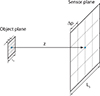 |
Fig. 1 Typical sampling scheme in lensless microscopy: The sensor plane and the object plane are separated by a distance z. The pixel pitch Δp in the sensor plane is larger than the pitch (resolution) d in the object plane. In the illustrated example, the factor between the grids is ρ = 4. The space bandwidth product of the system, i.e., the number of pixels N, is invariant. Consequently, the edge length of the sensor domain L S is larger than that of the object domain L O by a factor of ρ. |
with the numerical aperture NA = n · sin(α) and the wavelength λ. In the last step of equation (1) we have assumed the paraxial approximation sin(α) ≈ tan(α) = L S /(2z).
If light reflected or scattered by a specimen in the object plane is superposed with a reference wave R(x,y), the sensor will record an interference pattern (2)
(2)
where U H (x, y) denotes the complex hologram, i.e., the object wave across the sensor domain. We partly omitted the function arguments for the sake of readability. We can use any phase shifting method to extract the term M (x, y) = U H (x, y) · R * (x, y) from which we can obtain the complex hologram U H (x, y) if the structure of R is known.
To reconstruct the object wave field U
O
from the complex hologram U
H
we need to solve the inverse Rayleigh–Sommerfeld diffraction integral. Within the scalar diffraction theory, it provides an exact description of light propagation from a hologram plane x, y into an object plane u, v [26]: (3)
(3)
where  is the distance between two points in the hologram plane and the object plane.
Due to the finite aperture of the complex hologram U H the resolution of even the analytically exact solution for the reconstructed object wave field U O that equation (3) provides will always be limited by diffraction. We describe such a reconstruction as diffraction-limited. Consequently, a numerically exact solution to the inverse Rayleigh–Sommerfeld diffraction integral corresponds to a diffraction-limited reconstruction of the object wave field U O (u, v).
Initially, the Fresnel propagation formula readily comes to mind to solve equation (3). It is based on the Fresnel approximations that assume r ≈ z outside the exponentials, ik−1/r ≈ ik, and a first order binomial approximation of r within the exponentials![Mathematical equation: $$ r\approx z+\frac{1}{2z}\left[(x-u{)}^2+(y-v{)}^2\right]. $$](/articles/jeos/full_html/2026/01/jeos20250074/jeos20250074-eq5.gif) (4)
(4)
Its inverse propagates e.g., a measured wave field in the hologram plane U
H
(x, y) back into the object plane, as derived in [25], such that (5)
(5)
where F denotes the Fourier transform operator and S
1 and S
2 are two exponential functions with quadratic phase![Mathematical equation: $$ {S}_1=\mathrm{exp}\left[\frac{\mathrm{i}k\left({x}^2+{y}^2\right)}{2z}+\mathrm{i}{kz}\right]\hspace{1em}\mathrm{and}\hspace{1em}{S}_2=\mathrm{exp}\left[\frac{\mathrm{i}k\left({u}^2+{v}^2\right)}{2z}\right]. $$](/articles/jeos/full_html/2026/01/jeos20250074/jeos20250074-eq7.gif) (6)
(6)
The inverse Fresnel propagation formula has great advantages with respect to diffraction limited lensless imaging. It transforms a complex hologram sampled across the sensor grid, into an object wave field across a different sampling grid, whose pitch Δq = λz/L is approximately consistent with the diffraction limit d [1]. Hence, the Fresnel propagation formula inherently provides diffraction limited imaging. Unfortunately, since it is rooted in the Fresnel approximations, it only yields acceptable results for numerical apertures NA < 0.1, which makes it a mediocre choice for microscopy applications.
Precise reconstruction beyond this limit and without further pre-knowledge is not a simple task. The main problem is the high frequent chirp S
1 (x, y) in equation (5), which is substantially undersampled in the sensor domain. This, therefore, impedes the application of precise methods such as wave propagation by means of plane wave decomposition (or angular spectrum method). To realize this, we can write down the gradient of the phase ϕ (x, y) = arg{S
1}, e.g., in x-direction (7)
(7)
with k = 2π/λ being the wave vector. If we insert x = L
S
/2 to determine the highest phase gradient close to the sensors edges, we yield (8)
(8)
where we have used the Abbe diffraction limit equation (1) in the last step. As a result, we obtain approximately the Nyquist frequency ν N of the dense sampling grid in the object plane. Hence, S 1 is undersampled by a factor of approximately ρ in the sensor domain.
This has two major consequences which can be exemplified by the Wigner-space diagrams in Figure 2 that represent the space-bandwidth distribution of differently propagated wave fields (e.g., Fig. 2a shows the band-limited space-bandwidth of a wave field in the object plane): Firstly, as depicted in the Wigner-space diagram in Figure 2b, we cannot experimentally sample the wave field itself using the camera. The use of e.g., a plane reference wave would thus result in fringes too dense to be sampled by the finite-sized pixels. The pixels would average the high frequent parts of the interference pattern. Secondly, as shown in equation (8), if we do not know the entire wave field across the dense sampling grid, we cannot precisely reconstruct it. However, the wave field can be approximated across such a dense sampling grid through interpolation of the sparse hologram [27].
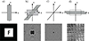 |
Fig. 2 Wigner-space diagrams as well as amplitude and phase images of a wave field throughout the lensless imaging process. ν is the bandwidth of the signal, while x is its lateral extent. a) Amplitude of wave field U O in the object plane, its support in phase space defines the space bandwidth-product (SBP) of the wave field. b) Phase of propagated wave field U H , the central box represents the SBP of a camera sensor. The propagation shears the support in phase space. High frequencies are recorded as badly sampled alias frequencies. c) Phase of propagated spherical reference wave R. d) Phase of the measured cross term M = U · R*, the spherical reference wave aligns the SBP of the coherence function and the sensor. |
2.2 Lensless Fourier holography
The solution to the first problem regarding sampling has been widely reported in the state of the art under the term Lensless Fourier Holography [28, 29]. The basic idea is to use a spherical reference wave R (x, y) which appears to originate from the center of the object, as shown in Figure 2c. This can be realized with a beam splitter for example. Since S
1 in equation (6) can be regarded as a parabolic approximation of a point source located in the center of the object as well, we can assume R ≈ S
1 for small numerical apertures. The measured cross term becomes  which can be sampled as shown in Figure 2d. In this situation, the reconstruction task reduces to a simple Fourier transform of M (x, y) as seen from equation (5), hence the name of the technique. The origin of the reference wave can also be laterally shifted to realize off-axis holography due to modulation of the interference pattern with a spatial carrier frequency. In this case, no additional phase shifting is required (single shot operation) to separate real and conjugate image. Additionally, the source of the reference wave, e.g., a fiber tip, can be placed next to the object, so that the beam splitter can be omitted.
A spherical reference wave works well to prevent averaging of frequencies during recording, but the assumption that the reconstruction process can be performed through a simple Fourier transform is still subject to the validity of equation (5) and therefore no more precise than the Fresnel propagation formula. Consequently, we need to find a more precise way to reconstruct the wave field in the object plane that does not rely on the Fresnel approximation.
2.3 Diffraction-limited reconstruction
In the following, we will solve the reconstruction problem in a two-step process, which is also shown schematically in the flow chart in Figure 3. Similarly to the scheme of lensless Fourier holography, we will assume the use of a spherical reference wave with known structure during recording. In the first step, we interpolate the measured cross term M (x, y). This is realized by Fourier transforming the cross term shown in Figure 3a into Fourier space shown in Figure 3b and applying zero-padding by a factor of ρ = Δp/d in Figure 3c, where Δp is the pixel pitch of the sensor and d is the diffraction limit. The zero-padding in Fourier space corresponds to a sinc-interpolation of the cross term M (x, y) which is a perfect reconstruction of the original function if the underlying cross term M (x, y) is band-limited [30]. This can be exemplified by the fact, that the Fourier transform of M (x, y) corresponds to propagating the wave field into the object plane by applying equation (5) and obtaining an approximate reconstruction of the object.
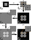 |
Fig. 3 Flowchart of the diffraction limited reconstruction process. The measured cross-term M(x, y) sampled across the sparse pixel grid of the camera sensor in a) is Fourier transformed (FT). Because of the Fourier holography scheme, the Fourier transform has the appearance of b) a (blurry) reconstruction of the object wave field U O and therefore centers the energy at the approximate location of the object across coordinates u = ξλz, v = ηλz. This blurry reconstruction is then zero-padded (ZP) in c) by the factor ρ = Δp/d, where Δp is the pixel pitch of the sensor and d is the diffraction limit. The zero-padded reconstruction is then Fourier transformed (FT−1) back into the hologram plane d). This results in a precise sinc-interpolated copy of the cross-term M in d). By multiplicative modulation with the analytical structure of the reference wave R(x,y) in e), the complex wave field U H is fully recreated in the sensor domain across the dense grid. The wave field is then precisely reconstructed using for example the angular spectrum method (ASM) f). |
While this procedure will result in a poor, blurry reconstruction which does not achieve full diffraction-limited resolution, the energy will still be confined close to the object support. Consequently, since the cross-term is band-limited the interpolated M does not feature any spurious defects such as aliasing. The result in Figure 3d will be an interpolated representation of M (x, y) across a sampling grid having the size of the sensor but the pitch of the object plane.
In the second step, we can now modulate the densely sampled M with the high frequent but known analytical structure of the reference wave R. This yields M · R = U H · R * · R = U H (assuming that the amplitude of the reference wave does not vary too much, so we can set |R| ≈ 1), thus digitally fully recreating the complex wave field U H in the sensor domain across the dense grid shown in Figure 3e. Now, we can simply employ the angular spectrum method [25] to yield an exact reconstruction of the complex wave field U O shown in Figure 3f.
To conclude, the two reconstruction steps do not include any approximations but are mathematically precise applications of the Rayleigh–Sommerfeld diffraction integral. Firstly, the sinc-interpolation of the complex hologram in Fourier space can not introduce any artifacts such as aliasing, since the complex hologram is band-limited, due to the Fourier holography setup. Secondly, the interpolated hologram is modulated with the analytical structure of the reference, while the subsequent propagation of the interpolated hologram via the angular spectrum method is mathematically equivalent to the application of the Rayleigh–Sommerfeld diffraction integral. This can exemplarily be seen in the exact reconstruction of the Siemens star shown in Figure 3f.
Because of the interpolation in the first reconstruction step, the computational complexity and runtime greatly depend on the desired feature size that shall be evaluated. For a N times N sized image and an interpolation ratio of ρ the reconstruction process consists of 1 FFT of a N × N matrix, 3 FFT of a ρ · N × ρ · N matrix and at least 2 multiplications of two ρ · N × ρ · N matrices. The algorithm is implemented in MATLAB to run on a CPU. Using a standard office computer with an Intel Core i7-5960X CPU, 3.00 GHz, the runtime of scenario realistic for industrial operation (N = 4512, ρ = 4) takes 35 s. For potential real-time operation, however computation times in the μs to ms range are ideal, a first step would be the implementation of the algorithm on a modern GPU.
3 Experimental results
3.1 Setup
As described above, to experimentally implement the proposed scheme for single shot sub-micron lensless microscopy a lensless Fourier holographic setup with a known reference wave is necessary. To allow for the wave field to be completely sampled, including all its high-frequent features necessary for full resolution, we consequently use a spherical reference wave with its origin approximately at the objects distance from the target.
We realized this in several setups both in transmission and reflection mode. Figures 4a, 4b show the main components as well as the light paths in transmission and reflection mode respectively. The reference source point is positioned slightly off-axis to allow for spatial phase shifting. In the reflection mode setup shown in Figure 4b the object illumination is generated by a lens, placed directly in front of the beam splitter. The reference source points for both transmission and reflection can be realized in multiple ways, e.g., using pinholes, tapered fiber tips (with high numerical aperture around NA ≈ 0.5) or by using microscope objectives to generate small focus points. In the following we demonstrate the technique both using tapered fiber tips as well as microscope objectives. Note that the term “lensless microscopy” here denotes the absence of lenses between object and camera. The utilized lenses are only used for beam shaping and do not directly influence the imaging or the resolution of the reconstruction.
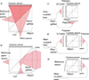 |
Fig. 4 Schematic illustrations of different implementations of the lensless holographic microscope in transmission mode (a + c) and reflection mode (b + d + e). a) and b) show the main components of the setup and the light paths similar to that of Fourier holography. The reference source point is off-axis to allow for spatial phase shifting. In reflection mode b) the object illumination (and potentially the reference wave) are generated by a lens, placed directly in front of the beam splitter. c-e) show concrete technical implementations of the lensless microscope. c) is a Mach–Zehnder interferometer implementation for transmission measurements. The polarization in both arms is aligned by a λ/2 plate and polarizers. d) shows a Mach–Zehnder interferometer implementation in reflection mode, while e) shows a Michelson interferometer implementation for reflection mode where the reference wave is generated by the same lens as the object illumination being reflected by a reference mirror. |
All measurements shown below were recorded with exposure times in or below the single digit ms range, making the single-shot measurement robust against mechanical vibrations. The camera gain was set to zero. Objects were positioned manually via micrometer precision stages. For off-axis measurements the temporal coherence length of the utilized lasers had to be at least in range of 500 μm to realize a modulation of the hologram with a spatial carrier frequency across the whole camera plane. The spatial coherence length has to be as large as the camera width, for fully modulated holograms. This can be realized by adjusting the choice of reference and object illumination source points described above.
The more detailed setup for transmission is shown in Figure 4c for measurements of e.g., biological samples and is based on a Mach–Zehnder-interferometer. The wave field from a fiber coupled laser is divided using a 50/50 fiber splitter (Thorlabs TW630R5F2) and recombined through a beam splitter after the object wave is diffracted by the object. Additionally, polarization filters are placed in both the object illumination and the reference arm of the interferometer to avoid degradation due to mismatched polarization. Potential degradations due to glare are effectively minimized by the use of diverging point sources. Problems due to reflections and ghost imaging caused by the beam splitter can be circumvented by using spatial phase shifting and masking the measured cross-term in Fourier-space. Therefore, no anti-reflective coating for the beam splitter is necessary.
In Figure 5 we see an example of a lensless microscopic image of a USAF resolution test chart in transmission. We used a CMOS camera with a Sony IMX661 sensor, containing 13376 times 9528 pixels with a pitch of 3.45 μm, a frequency-double Nd:YAG laser at λ = 532 nm, and a beam splitter cube with 50 mm side lengths. The point sources were generated using microscope objectives. The field of view is approx. 7 × 7 mm2 and from the detail we see that the resolution is approx. 1.5 μm (group 8, 3rd element), well below the pixel pitch. This corresponds to diffraction limited imaging with a numerical aperture of N A = 0.25 over a comparably large field of view. The space bandwidth-product (SBP) of the image is more than 20 million, which is remarkable considering that typical microscope objectives achieve SBPs between 9 and 15 million.
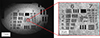 |
Fig. 5 USAF resolution target measured by means of lensless holographic microscopy in transmission mode: The field of view is approx. 7 × 7 mm2, whereas the resolution is approx. 1.5 μm at group 8 element 3 as shown in the blow up. The image therefore has a remarkably high space-bandwidth product of more than 20 million. |
For even lower resolutions around the diffraction limit, a high signal-to-noise ratio is paramount. One way to achieve higher signal-to-noise ratios is to place the source point of the object illumination close to the object itself, thus illuminating just a smaller area, which in turn results in a smaller field of view in the reconstruction. For this, we used a HeNe laser with a wavelength of λ = 632.8 nm as the light source. A CMOS camera with a Sony IMX541 sensor with dimensions of 5120 × 5120 pixels and a pixel pitch of 2.5 μm serves for imaging. However, the effective sensor length is constrained to L = 12.5 mm by the beam splitter. With the distance between object and camera being 16 mm and a refractive index of the beam splitter of n ≈ 1.5, the numerical aperture of the setup is NA = 0.55.
The numerical aperture corresponds to a diffraction limit of δ = 0.57 μm. To find the actual resolution of the setup we recorded a digital hologram of a USAF MIL-STD 150A resolution chart. The hologram was reconstructed using the propagation algorithm shown in Figure 3, with the result shown in Figure 6a. The smallest available element of group 9 is fully resolved which indicates an optical resolution of below 0.78 μm. For reference the red square indicates the size of a 2.5 μm camera pixel.
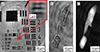 |
Fig. 6 a) Holographic reconstruction of a USAF MIL-STD 150A resolution chart measured in transmission. The smallest available group 9, element 3 with a line width of 0.78 μm is fully resolved as can be seen in the blow up. For reference, the red square indicates the size of a 2.5 μm camera pixel. Holographic reconstruction of the amplitude b) and unwrapped phase contrast c) of pancreas cells of the PANC-1 cell line. The cell morphology including the nucleus and cell organelle are resolved. |
Additionally, we demonstrate the capability to image biological samples on PANC-1 cells, a human pancreatic carcinoma cell line, with an average diameter of approximately 10–50 μm, which were suspended in culture medium and seeded onto a petri dish. As expected the cell morphology shown in Figures 6b, 6c is resolved, with observable cell cores and organelles.
For the measurement in reflection mode, e.g., for quality insurance in wafer testing, we used two types of setup, shown in Figures 4d, 4e. The setup in d also resembles that of a Mach–Zehnder interferometer as described for transmission mode, except for the object illumination. The setup in Figure 4e is in a Michelson interferometer configuration, where the reference wave is generated by reflection at a reference mirror.
We tested the achievable resolution in reflection mode using a resolution chart as well. For a higher signal-to-noise ratio and to achieve the highest possible resolution we measured the digital hologram via temporal phase-shifting in the setup shown in Figure 4e. We used a CMOS camera with a Sony IMX541 sensor with 4512 × 4512 pixels with a pixel pitch of 2.74 μm and a supercontinuum white light laser (NKT Photonics Fianium, SuperK VARIA) at 532 nm for a shorter coherence length and thus less coherent noise. While the diffraction limited resolution given by the numerical aperture is δ ≈ 0.53 μm the smallest resolved elements of the reconstructed resolution chart in Figure 7a have a line width of 0.98 μm. Consequently, we did not achieve diffraction-limited resolution in reflection. The difference in resolution can likely be attributed to distortion stemming from the lens that generates the spherical reference wave and spherical aberrations from the beam splitter cube.
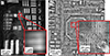 |
Fig. 7 Holographic reconstructions of a) a USAF resolution chart and b) an MEMS chip measured in reflection mode. The smallest resolved elements (group 9, element 1) of the resolution target have a line width of 0.98 μm. The reconstruction of the MEMS achieves a resolution of at least 2 μm and shows that capacitors and springs in the single-digit micrometer range can be resolved across a field of view of around 2.5 mm. |
To demonstrate the techniques capability in technical applications such as wafer level testing, we furthermore recorded a hologram of a micro-electronic-mechanical system (MEMS) acceleration sensor which contains object features in the low single digit micrometer range. The reference source point was generated using a tapered, lensed single mode fiber (by InZiv LTD) with a spot diameter of 0.8 μm and a working distance of 4 μm. As shown in Figure 7b the capacitors and piezoresistors with sizes of a few micrometers can be resolved across the whole field of view of 2.5 mm diameter. The MEMS sensor was measured in a single-shot measurement, using spatial phase-shifting due to the off-axis holographic setup.
For a quantitative evaluation of the resolution in both transmission and reflection mode we computed the modulation transfer function (MTF) in Figure 8 exemplarily for the reconstructions of the USAF resolution charts shown in Figures 6a and 7a respectively. For this, we evaluated the mean Michelson contrast C = (I max − I min)/(I max + I min) for the resolved resolution bar triplets. The normalized MTF of the transmission measurement stays above or around 0.9 up to resolutions of 456 line pairs per mm (lp/mm) and drops only to 0.71 ± 0.04 for the smallest available line pairs (645 lp/mm, 0.78 μm linewidth). This indicates that a higher resolution might be achievable if smaller elements were available. The MTF in reflection mode however is significantly lower with values of 0.22 ± 0.02 at 512 lp/mm. This is likely due to wavefront errors in the reference wave.
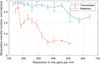 |
Fig. 8 Modulation transfer function (MTF), representing the mean Michelson contrast, evaluated exemplarily for the reconstructions in transmission and reflection mode of the USAF resolution charts shown in Figures 6a and 7a. The MTF of the transmission measurement remain relatively high for all available resolution groups. The MTF in reflection mode is significantly lower, likely due to wavefront errors in the reference wave. The dip around 200 line pairs per mm in reflection mode can likely be attributed to degradations of elements close to the edge of the illuminated aperture and is otherwise not significant. The error bars represent the standard deviation across individual bars in Figures 6a and 7a respectively. |
A comparison with the state of the art of lensless microscopic techniques shows, that, while single shot techniques such as lensless inline holography using iterative phase retrieval have the same robustness as our proposed technique, computation times can also be high, in the second to minutes range [31, 32]. However, the main drawback of these techniques, is the limitation of resolution to the pixel pitch, which we can easily overcome. Multi-shot holography and pixel-super-resolution techniques instead are able to reach resolutions down to the diffraction limit and reach real time reconstruction using deep neural networks [33, 34, 35]. Since these techniques need multiple measurements to achieve sub-pixel resolution, they however do not have same robustness as single shot measurements, which limits their applicability to transient processes.
4 Conclusion and outlook
We have developed a novel reconstruction process for diffraction-limited lensless holographic microscopy utilizing the inherent sampling pitch transformation of the Fresnel propagation for an initial spatially limited reconstruction of the hologram. This initial reconstruction, however, will always be severely degraded by the Fresnel approximation and is consequently only used to interpolate the hologram by zero-padding the Fresnel reconstruction and propagating the zero-padded signal back into the hologram plane. The interpolated hologram with a pixel pitch corresponding to the diffraction limit can now be propagated into the object plane again using any exact wave field propagator, such as the angular spectrum method.
Using single-shot measurements, we achieve a resolution of approx. 1.5 μm across a field of view of approx. 7 × 7 mm2, corresponding to a space bandwidth-product of 20 million, surpassing many conventional microscope objectives. A resolution below 1 μm, close to the diffraction limit requires higher signal-to-noise ratios which we achieve by using temporal instead of spatial phase shifting in reflection mode and by limiting the illuminated object area and thus the field of view to a few 100 μm. We record a lateral resolution of 0.78 μm in transmission mode and 0.98 μm in reflection mode. The difference in resolution between transmission and reflection is likely due to aberrations of the reference wave, which is assumed to be spherical. In reflection mode, the reference wave is submitted to greater degradations than in transmission mode. Especially for the measurement of the resolution target, the reference wave is generated by an additional lens in front of the beam splitter, which is reflected by a reference mirror behind the beam splitter. Consequently, the reference wave is degraded by spherical aberrations due to the double transmission through the beam splitter as well as degradations from imperfections of the lens and its alignment.
The reconstruction process assumes a perfectly spherical reference wave. To achieve diffraction limited resolution in both transmission and reflection modes across larger fields of view, additional calibration of the reference wave is needed. For this, we will implement an additional wavefront measurement using, e.g., a Shack–Hartmann sensor or computational shear-interferometry [36] in future research. The measured wavefront errors, differing from an ideal spherical wave, can be digitally compensated. Initial simulations show that compensating wavefront errors would allow for sub-micron resolution across several mm to cm diameter fields of view.
An alternative way to reduce degradations of the reference wave is to use a lensless holographic Gabor configuration for measurements in transmission mode. Using a single light source the non-diffracted light acts as a reference wave. This would especially eliminate degradations stemming from beam splitters. Future investigations will include transmission measurements in Gabor configuration.
Funding
The authors gratefully acknowledge the support of the Deutsche Forschungsgemeinschaft (DFG, German Research Foundation) for funding this work under the project “HyperCOMet”, grant no. 430572965.
Conflicts of interest
The authors declare no conflicts of interest.
Data availability statement
The Data underlying the presented results and the used Matlab algorithms may be obtained from the authors upon a reasonable request.
Author contribution statement
Conceptualization, C.F.; Data curation, A.F.M. and C.F.; Investigation, A.F.M., J.A.B.; Methodology, A.F.M. and C.F.; Validation, A.F.M., J.A.B. and C.F.; Visualization, A.F.M., J.A.B. and C.F..; Formal Analysis, A.F.M. and C.F.; Writing – original draft, A.F.M., and C.F.; Funding acquisition, R.B.B.; Supervision and discussion of results, R.B.B. and C.F. All authors have read and agreed to the submitted version of the manuscript.
Acknowledgments
The authors thank Manfred Radmacher (Universität Bremen) for sharing PANC1 cells and Sander van der Driesche (Universität Bremen) for preparing the PANC1 cells for measurement, as well as Reiner Klattenhoff and Bennet Wucherpfennig for their support with the experimental measurements.
References
- Schnars U, Falldorf C, Watson J, Jüptner W, Digital holography and wavefront sensing (Springer, 2015). [Google Scholar]
- Falldorf C, Thiemicke F, Müller AF, Agour M, Bergmann RB, Flash-profilometry fullfield lensless acquisition of spectral holograms for coherence scanning profilometry, Opt. Expr. 31(17), 27494–27507 (2023). [Google Scholar]
- de Groot PJ, Deck LL, Su R, Osten W, Contributions of holography to the advancement of interferometric measurements of surface topography, Light: Adv. Manuf. 3(1), 1–20 (2022). [Google Scholar]
- Fratz M, Seyler T, Bertz A, Carl D, Digital holography in production: an overview, Light: Adv. Manuf. 2(3), 283–295 (2021). [Google Scholar]
- Balasubramani V, Kuś A, Tu HY, Cheng CJ, Baczewska M, Krauze W, et al., Holographic tomography: techniques and biomedical applications, Appl. Opt. 60(10), B65–B80 (2021). [Google Scholar]
- An J, Won K, Kim Y, Hong JY, Kim H, Kim Y, et al., Slim-panel holographic video display, Nat. Commun. 11(1), 5568 (2020). [Google Scholar]
- Falldorf C, Rukin I, Müller AF, Kroker S, Bergmann RB, Functional pixels: a pathway towards true holographic displays using today’s display technology, Opt. Expr. 30(26), 47528–47540 (2022). [Google Scholar]
- Ozcan A, McLeod E, Lensless imaging and sensing, Annu. Rev. Biomed. Eng. 18, 77–102 (2016). [Google Scholar]
- Kim J, Lee SJ, Digital in-line holographic microscopy for label-free identification and tracking of biological cells, Mil. Med. Res. 11(1), 38 (2024). [Google Scholar]
- Boominathan V, Robinson JT, Waller L, Veeraraghavan A, Recent advances in lensless imaging, Optica. 9(1), 1–16 (2022). [Google Scholar]
- Falldorf C, Müller AF, Pazos BGC, Bich JA, Bergmann RB, Current progress in lensless holographic microscopy, in 3D Imag Visual Disp., Vol. 13465 (SPIE, 2025), pp. 19–26. [Google Scholar]
- Tobon-Maya H, Zapata-Valencia S, Zora-Guzmán E, Buitrago-Duque C, Garcia-Sucerquia J, Open-source, cost-effective, portable, 3D-printed digital lensless holographic microscope, Appl. Opt. 60(4), A205–A214 (2021). [Google Scholar]
- Chen D, Wang L, Luo X, Xie H, Chen X, Resolution and contrast enhancement for Lensless digital holographic microscopy and its application in biomedicine, Photonics 9(5), 358 (2022). [Google Scholar]
- Gao P, Yuan C, Resolution enhancement of digital holographic microscopy via synthetic aperture: a review, Light: Adv. Manuf. 3(1), 105–120 (2022). [Google Scholar]
- Massig JH, Digital off-axis holography with a synthetic aperture, Opt. Lett. 27(24), 2179–2181 (2002). [Google Scholar]
- Greenbaum A, Zhang Y, Feizi A, Chung PL, Luo W, Kandukuri SR, et al., Wide-field computational imaging of pathology slides using lens-free on-chip microscopy, Sci. Transl. Med. 6(267), 267ra175–5 (2014). [Google Scholar]
- Bianco V, Paturzo M, Ferraro P, Spatio-temporal scanning modality for synthesizing interferograms and digital holograms, Opt. Expr. 22(19), 22328–22339 (2014). [Google Scholar]
- Su TW, Isikman SO, Bishara W, Tseng D, Erlinger A, Ozcan A, Multi-angle lensless digital holography for depth resolved imaging on a chip, Opt. Expr. 18(9), 9690–9711 (2010). [Google Scholar]
- Paturzo M, Merola F, Grilli S, De Nicola S, Finizio A, Ferraro P, Super-resolution in digital holography by a two-dimensional dynamic phase grating, Opt. Expr. 16(21), 17107–17118 (2008). [Google Scholar]
- Shimobaba T, Kakue T, Ito T, Review of fast algorithms and hardware implementations on computer holography, IEEE Trans. Ind. Inf. 12(4), 1611–1622 (2015). [Google Scholar]
- Müller AF, Bergmann RB, Falldorf C, High resolution lensless microscopy based on Fresnel propagation, Opt. Eng. 63(11), 111805–111815 (2024). [Google Scholar]
- Restrepo JF, Garcia-Sucerquia J, Magnified reconstruction of digitally recorded holograms by Fresnel–Bluestein transform, Appl. Opt. 49(33), 6430–6435 (2010). [Google Scholar]
- Li JC, Tankam P, Peng ZJ, Picart P, Digital holographic reconstruction of large objects using a convolution approach and adjustable magnification, Opt. Lett. 34(5), 572–574 (2009). [NASA ADS] [CrossRef] [Google Scholar]
- Heintzmann R, Loetgering L, Wechsler F, Scalable angular spectrum propagation, Optica 10(11), 1407–1416 (2023). [Google Scholar]
- Goodman JW, Introduction to Fourier optics (Roberts and Company Publishers, 2005). [Google Scholar]
- Nascov V, Logofătu PC, Fast computation algorithm for the Rayleigh–Sommerfeld diffraction formula using a type of scaled convolution, Appl. Opt. 48(22), 4310–4319 (2009). [Google Scholar]
- Pedrini G, Schedin S, Tiziani HJ, Aberration compensation in digital holographic reconstruction of microscopic objects, J. Modern Opt 48(6), 1035–1041 (2001). [Google Scholar]
- Wagner C, Seebacher S, Osten W, Jüptner W, Digital recording and numerical reconstruction of lensless Fourier holograms in optical metrology, Appl. Opt. 38(22), 4812–4820 (1999). [CrossRef] [Google Scholar]
- Mustafi S, Latychevskaia T, Fourier transform holography: A lensless imaging technique, its principles and applications, Photonics 10(2), 153 (2023). [Google Scholar]
- Yaroslavsky L, Boundary effect free and adaptive discrete signal sinc-interpolation algorithms for signal and image resampling, Appl. Opt. 42(20), 4166–4175 (2003). [Google Scholar]
- Galande AS, Gurram HPR, Kamireddy AP, Venkatapuram VS, Hasan Q, John R, Quantitative phase imaging of biological cells using lensless inline holographic microscopy through sparsity-assisted iterative phase retrieval algorithm, J. Appl. Phys. 132(24), 243102 (2022). [Google Scholar]
- Guo C, Liu X, Zhang F, Du Y, Zheng S, Wang Z, et al., Lensfree on-chip microscopy based on single-plane phase retrieval, Opt. Expr. 30(11), 19855–19870 (2022). [Google Scholar]
- De Haan K, Rivenson Y, Wu Y, Ozcan A, Deep-learning-based image reconstruction and enhancement in optical microscopy, Proc. IEEE 108(1), 30–50 (2019). [Google Scholar]
- Lee H, Sung J, Park S, Shin J, Kim H, Kim W, et al., Lens-free reflective topography for high-resolution wafer inspection, Sci. Rep. 14(1), 10519 (2024). [Google Scholar]
- Wu X, Zhou N, Chen Y, Sun J, Lu L, Chen Q, et al., Lens-free on-chip 3D microscopy based on wavelength-scanning Fourier ptychographic diffraction tomography, Light: Sci. Appl. 13(1), 237 (2024). [Google Scholar]
- Falldorf C, Agour M, Bergmann RB, Digital holography and quantitative phase contrast imaging using computational shear interferometry, Opt. Eng. 54(2), 024110 (2015). [Google Scholar]
All Figures
|
Fig. 1 Typical sampling scheme in lensless microscopy: The sensor plane and the object plane are separated by a distance z. The pixel pitch Δp in the sensor plane is larger than the pitch (resolution) d in the object plane. In the illustrated example, the factor between the grids is ρ = 4. The space bandwidth product of the system, i.e., the number of pixels N, is invariant. Consequently, the edge length of the sensor domain L S is larger than that of the object domain L O by a factor of ρ. |
| In the text | |
|
Fig. 2 Wigner-space diagrams as well as amplitude and phase images of a wave field throughout the lensless imaging process. ν is the bandwidth of the signal, while x is its lateral extent. a) Amplitude of wave field U O in the object plane, its support in phase space defines the space bandwidth-product (SBP) of the wave field. b) Phase of propagated wave field U H , the central box represents the SBP of a camera sensor. The propagation shears the support in phase space. High frequencies are recorded as badly sampled alias frequencies. c) Phase of propagated spherical reference wave R. d) Phase of the measured cross term M = U · R*, the spherical reference wave aligns the SBP of the coherence function and the sensor. |
| In the text | |
|
Fig. 3 Flowchart of the diffraction limited reconstruction process. The measured cross-term M(x, y) sampled across the sparse pixel grid of the camera sensor in a) is Fourier transformed (FT). Because of the Fourier holography scheme, the Fourier transform has the appearance of b) a (blurry) reconstruction of the object wave field U O and therefore centers the energy at the approximate location of the object across coordinates u = ξλz, v = ηλz. This blurry reconstruction is then zero-padded (ZP) in c) by the factor ρ = Δp/d, where Δp is the pixel pitch of the sensor and d is the diffraction limit. The zero-padded reconstruction is then Fourier transformed (FT−1) back into the hologram plane d). This results in a precise sinc-interpolated copy of the cross-term M in d). By multiplicative modulation with the analytical structure of the reference wave R(x,y) in e), the complex wave field U H is fully recreated in the sensor domain across the dense grid. The wave field is then precisely reconstructed using for example the angular spectrum method (ASM) f). |
| In the text | |
|
Fig. 4 Schematic illustrations of different implementations of the lensless holographic microscope in transmission mode (a + c) and reflection mode (b + d + e). a) and b) show the main components of the setup and the light paths similar to that of Fourier holography. The reference source point is off-axis to allow for spatial phase shifting. In reflection mode b) the object illumination (and potentially the reference wave) are generated by a lens, placed directly in front of the beam splitter. c-e) show concrete technical implementations of the lensless microscope. c) is a Mach–Zehnder interferometer implementation for transmission measurements. The polarization in both arms is aligned by a λ/2 plate and polarizers. d) shows a Mach–Zehnder interferometer implementation in reflection mode, while e) shows a Michelson interferometer implementation for reflection mode where the reference wave is generated by the same lens as the object illumination being reflected by a reference mirror. |
| In the text | |
|
Fig. 5 USAF resolution target measured by means of lensless holographic microscopy in transmission mode: The field of view is approx. 7 × 7 mm2, whereas the resolution is approx. 1.5 μm at group 8 element 3 as shown in the blow up. The image therefore has a remarkably high space-bandwidth product of more than 20 million. |
| In the text | |
|
Fig. 6 a) Holographic reconstruction of a USAF MIL-STD 150A resolution chart measured in transmission. The smallest available group 9, element 3 with a line width of 0.78 μm is fully resolved as can be seen in the blow up. For reference, the red square indicates the size of a 2.5 μm camera pixel. Holographic reconstruction of the amplitude b) and unwrapped phase contrast c) of pancreas cells of the PANC-1 cell line. The cell morphology including the nucleus and cell organelle are resolved. |
| In the text | |
|
Fig. 7 Holographic reconstructions of a) a USAF resolution chart and b) an MEMS chip measured in reflection mode. The smallest resolved elements (group 9, element 1) of the resolution target have a line width of 0.98 μm. The reconstruction of the MEMS achieves a resolution of at least 2 μm and shows that capacitors and springs in the single-digit micrometer range can be resolved across a field of view of around 2.5 mm. |
| In the text | |
|
Fig. 8 Modulation transfer function (MTF), representing the mean Michelson contrast, evaluated exemplarily for the reconstructions in transmission and reflection mode of the USAF resolution charts shown in Figures 6a and 7a. The MTF of the transmission measurement remain relatively high for all available resolution groups. The MTF in reflection mode is significantly lower, likely due to wavefront errors in the reference wave. The dip around 200 line pairs per mm in reflection mode can likely be attributed to degradations of elements close to the edge of the illuminated aperture and is otherwise not significant. The error bars represent the standard deviation across individual bars in Figures 6a and 7a respectively. |
| In the text | |
Current usage metrics show cumulative count of Article Views (full-text article views including HTML views, PDF and ePub downloads, according to the available data) and Abstracts Views on Vision4Press platform.
Data correspond to usage on the plateform after 2015. The current usage metrics is available 48-96 hours after online publication and is updated daily on week days.
Initial download of the metrics may take a while.