| Issue |
J. Eur. Opt. Society-Rapid Publ.
Volume 22, Number 1, 2026
EOSAM 2025
|
|
|---|---|---|
| Article Number | 13 | |
| Number of page(s) | 5 | |
| DOI | https://doi.org/10.1051/jeos/2026008 | |
| Published online | 27 February 2026 | |
Short Communication
Modeling of surface vessels using distributed acoustic sensing data and physics-based optimization
1
INESC TEC – Instituto de Engenharia de Sistemas e Computadores, Tecnologia e Ciência, Rua Dr. Roberto Frias, 4200-465 Porto, Portugal
2
Faculdade de Ciências da Universidade do Porto, Rua do Campo Alegre s/n, 4169-007 Porto, Portugal
3
Instituto Hidrográfico, Rua das Trinas 49, 1249-093 Lisboa, Portugal
* Corresponding author: This email address is being protected from spambots. You need JavaScript enabled to view it.
Received:
15
December
2025
Accepted:
25
January
2026
Abstract
Technological advances in global communications depend significantly on robust and efficient long-distance infrastructures. One notable example is the submarine cable network. Installed on the ocean floor, these cables use fiber optic technology to transmit large volumes of data at high speed and low latency between continents. Beyond their primary communication function, recent innovations allow these cables to serve as Distributed Acoustic Sensing (DAS) systems, effectively converting tens of kilometers of passive fiber into massive, coherent arrays of vibration sensors. The primary objective of this project is to enhance maritime surveillance capabilities by integrating DAS technology with advanced kinematic modeling. This paper establishes a rigorous physical and mathematical framework for interpreting the acoustic signatures of surface vessels detected by bottom-mounted fibers. We derive the complete opto-acoustic transfer function, formulate the hyperbolic moveout equations based on a moving point-source solution to the wave equation, and implement a stochastic inversion scheme using Differential Evolution. By optimizing a correlation-based loss function, we demonstrate the ability to recover vessel trajectory, speed, and depth from complex interferometric patterns with speed estimation errors consistently below 1%. This approach allows for the extraction of quantitative physical parameters from raw optical data, bridging the gap between photonics and hydroacoustics.
Key words: Distributed acoustic sensing / Maritime surveillance / ϕ-OTDR / Hyperbolic moveout / Differential evolution / Optimization
© The Author(s), published by EDP Sciences, 2026
 This is an Open Access article distributed under the terms of the Creative Commons Attribution License (https://creativecommons.org/licenses/by/4.0), which permits unrestricted use, distribution, and reproduction in any medium, provided the original work is properly cited.
1 Introduction
Distributed Acoustic Sensing (DAS) has revolutionized the field of optical monitoring by enabling the conversion of standard fiber optic cables into large-scale, ultra-sensitive vibration sensor arrays [1, 2]. Originally developed for vertical seismic profiling and pipeline monitoring within the oil and gas industry, DAS technology is now finding critical applications in environmental monitoring and critical infrastructure security. Specifically, submarine telecommunication cables can be repurposed as distributed seismic or acoustic sensors, providing meter-scale spatial resolution and continuous coverage over tens of kilometers of the ocean floor [3, 4]. Recent studies have demonstrated that DAS is capable of detecting underwater hydroacoustic signals, including the mechanical noise generated by surface vessels, with performance metrics comparable to conventional hydrophone arrays, although the Signal-to-Noise Ratio (SNR) may vary across frequency bands [5].
The primary challenge in transforming a DAS system into a reliable vessel tracking platform lies in the complexity of the signal processing required. As a ship moves through the water, it generates continuous acoustic noise resulting from engine vibrations and propeller cavitation. Because the ship moves relative to the stationary fiber on the seabed, these acoustic wavefronts reach different sections of the fiber at different times, producing distinct, geometry-dependent patterns in the recorded data. This paper presents a comprehensive mathematical formulation of these hyperbolic moveout patterns and introduces an inverse problem framework designed to extract precise vessel movement and physical characteristics directly from raw DAS waterfall plots.
Unlike prior studies, which have primarily focused on the simple detection or qualitative visualization of vessel signatures, our approach enables the quantitative inference of vessel dynamics and physical parameters from DAS measurements. Global maritime security currently relies heavily on Automatic Identification System (AIS) transponders [6]. However, AIS data is inherently vulnerable to spoofing, can be deliberately disabled by “dark vessels,” or may be unavailable in remote ocean areas due to sparse receiver coverage. Consequently, there is a critical need for passive, non-cooperative surveillance systems that do not rely on the target’s participation. Submarine cables, which already crisscross the world’s oceans, offer an ideal, covert platform for this purpose [7]. By connecting a DAS interrogator to dark fiber strands, real-time acoustic monitoring can be achieved over vast distances with high resolution. This work presents a rigorous physical–mathematical framework for the acoustic detection of surface vessels using bottom-mounted optical fibers, deriving the opto-acoustic transfer function and hyperbolic moveout equations from the wave equation for a moving point source, and solving the inversion using a Differential Evolution–based stochastic optimization strategy.
2 Physical principles of phase-sensitive OTDR
To interpret the acquired data, we model the Phase-sensitive Optical Time Domain Reflectometry (ϕ-OTDR) process [2]. The fiber acts as a one-dimensional waveguide with random scattering centers. As a coherent laser pulse propagates, the backscattered electric field is formed by the superposition of contributions from scatterers within the pulse width.
When an external acoustic pressure wave P(r, t) interacts with the cable, it induces a mechanical strain on the fiber core. In DAS, we measure the differential phase shift Δϕ between two sections of fiber separated by a gauge length L
g
. Assuming the acoustic wavelength is larger than the gauge length, the relationship between the recorded optical phase and the axial dynamic strain ϵ
zz is linear: (1)
(1)
where ξ ≈ 0.78 is the photo-elastic scaling factor and n is the refractive index. This establishes that the recorded optical phase is a direct proxy for the strain induced by the vessel’s acoustic emission.
3 Kinematic and acoustic wavefield modeling
We model the ocean as a semi-infinite homogeneous half-space and the vessel as a moving point source emitting a broadband signal S(t).
3.1 Hyperbolic moveout and directional sensitivity
For a vessel moving with velocity v
s
along a linear trajectory at the surface, the acoustic arrival time at the fiber creates a hyperbola: (2)
(2)
where t CPA is the time at the Closest Point of Approach (CPA) and V app is the moveout velocity. This relationship allows us to invert the vessel speed and impact parameter from the data curvature. Additionally, the fiber acts as a dipole sensor; its sensitivity to axial strain results in a characteristic amplitude “null” when the acoustic wavefronts arrive perpendicular to the cable (at CPA), facilitating precise localization [8].
3.2 Spectral interference and Doppler effects
Beyond kinematics, the signal contains spectral features derived from the source depth and motion. The interaction between the direct acoustic path and the surface reflection (Lloyd’s Mirror effect) creates frequency notches dependent on the source depth z s . Simultaneously, the broadband noise undergoes a Doppler shift due to the relative radial velocity, resulting in a sigmoidal frequency transition. These physical constraints – interference patterns and Doppler shifts – are critical for validating estimated velocities and depths [9].
3.3 Numerical implementation
To validate the model, we implemented a numerical forward model that synthesizes the DAS waterfall plot D(x, t). The simulation procedure is summarized in Algorithm 1. It generates a parametric source S(t) composed of a fundamental frequency and harmonics, modulated by Lloyd’s Mirror interference. The source is spatially windowed by a geometric hull function to simulate the acoustic wake, scaled by geometrical spreading, and finally convolved with the gauge length operator to replicate the physical measurement process.
1: Input: Grid (x, t), Vessel Params m
2: Output: Synthesized Data Matrix D(x, t)
3: Initialize D ← 0
4: for each time step tj do
5: Calculate vessel position  using
using 
6: for each sensor channel xi do
7: Compute range 
8 Compute Doppler factor fDop and Arrival Time tarr
9: Spectral Source: 
10: Interference: Apply Lloyd’s Mirror modulation
11: Hull Window: Apply spatial envelope H(l)
12: Spreading: Scale by 
13: Accumulate strain: 
14: end for
15: end for
16: Sensor Model: Convolve D with Gauge Length Lg
17: Return D
4 Inverse problem and optimization strategy
Inverting kinematic parameters from DAS data is a non-linear optimization problem complicated by oscillatory interference patterns and the hyperbolic nature of the moveouts. To avoid the local minima that are inherent to gradient-based methods in such rugged landscapes, we employed Differential Evolution (DE) [10], a robust stochastic global optimization algorithm. The vessel state is defined by the parameter vector m = [v s , θ 0, z s , f 0, L s , W s,γ ]T, representing the speed, angular offset, source depth, fundamental frequency, vessel length, vessel width, and spreading coefficient, respectively. The search space is bounded by physically constrained limits (e.g., v s ∈ [1, 20] m/s) to ensure the algorithm converges to realistic solutions.
Using a classic DE/rand/1/bin strategy, the algorithm evolves a population of candidate vectors over successive generations. A mutant vector  is generated for each target vector
  by mixing three random population members:
 (3)
(3)
where F is the differential scaling factor. Binomial crossover is then performed to create a trial vector, which replaces the target vector only if it yields an improvement in the objective function.
To address the lack of absolute amplitude calibration in DAS data (which can vary due to fiber coupling and signal fading), we chose to optimize for structural similarity rather than absolute intensity. We minimize a correlation-based loss function  :
: (4)
(4)
where S(m) is the simulated field generated by the candidate parameters, R is the observed experimental data, and σ denotes the standard deviation. This scale-invariant metric ensures the model locks onto geometric features – such as the hyperbolic curvature and interference nulls – independent of the overall signal magnitude.
5 Material and methods
5.1 Data acquisition
The experimental data was acquired using a standard commercial DAS interrogator unit connected to a bottom-mounted submarine telecommunications cable. The interrogator’s pulse repetition rate yielded a temporal sampling frequency f s sufficient to capture the acoustic spectrum of vessel noise, while the optical gauge length L g provided a spatial sampling resolution of approximately 9.8 m.
5.2 Signal preprocessing pipeline
Before the optimization process, the raw optical phase data undergoes a rigorous, multi-stage preprocessing pipeline designed to maximize the Signal-to-Noise Ratio (SNR) and ensure statistical consistency with the forward model. Raw DAS data is typically dominated by high-amplitude, low-frequency environmental noise, such as ocean swell and hydrostatic pressure variations (<1 Hz). To isolate the specific mechanical signature of the vessel, we applied an 8th-order Butterworth bandpass filter with a passband of [2, 120] Hz. This range was selected to capture the fundamental engine harmonics and propeller blade pass frequencies while effectively rejecting microseisms and high-frequency system noise.
Following filtration, we addressed the computational constraints imposed by the high sampling rates of DAS systems. We performed temporal decimation immediately following the anti-aliasing filter to reduce the computational load of the fitness evaluation function. For datasets with high SNR (Case B), the raw coherent strain was used directly. However, for lower SNR scenarios (Case A), we computed the Hilbert envelope of the signal. This transformation focuses the optimizer on the energy distribution of the acoustic arrival rather than the rapidly oscillating phase carrier, significantly improving convergence stability in noise-limited regimes. Finally, because the correlation-based loss function requires that the simulated and experimental data share comparable statistical properties, we applied a Z-score standardization to the preprocessed data matrix D, subtracting the global mean μ D and dividing by the standard deviation σ D . To prevent transient artifacts (e.g., system glitches or dropped channels) from skewing the correlation metric, the data was robustly clipped to the 99th percentile. This ensures the optimization surface remains smooth and gradients are driven by the persistent vessel wake geometry.
6 Results
The efficacy of the proposed model was assessed via wavefield reconstruction and validation against independent AIS ground-truth data (Table 1). Figure 1 demonstrates the high fidelity of the model in reproducing the signal topology for both test cases (Fig. 2).
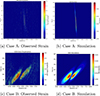 |
Figure 1 Comparative validation of the forward model against experimental DAS data. Top row (a, b): Case A (Mestre Horácio), showing strong, coherent hyperbolic arrivals. Bottom row (c, d): Case B (Wilson Hirtshals), where the simulation accurately reconstructs the fainter interference lobules (Lloyd’s Mirror effect), providing visual confirmation of the source depth estimation. |
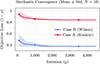 |
Figure 2 Stochastic convergence of the Differential Evolution algorithm (N = 10 runs). The solid lines represent the mean best loss (1 − ρ) as a function of generation, and the shaded areas indicate ±1 standard deviation. Case B (blue) converges to a significantly lower residual (≈0.38) with high stability, while Case A (red) stabilizes at a higher noise floor (≈0.84). |
Inverted kinematic parameters and validation against AIS (Mean ± SD over 10 independent runs).
7 Conclusion
This work has successfully established a comprehensive physics-based framework for vessel tracking using Distributed Acoustic Sensing (DAS) combined with Differential Evolution optimization. We have demonstrated the ability to recover critical kinematic parameters (speed, trajectory, depth) and vessel dimensions from raw interferometric data, confirming the viability of repurposing existing single-mode submarine cables as massive, distributed hydrophone arrays. The proposed optimization scheme proved to be robust against varying levels of environmental noise, accurately resolving complex hyperbolic moveout features and interference patterns. Specifically, we achieved velocity estimation errors below 1% in high-SNR conditions. Future work will focus on integrating these kinematic priors into deep learning architectures, aiming to develop fully automated, real-time maritime surveillance systems.
Funding
This work is supported by Component 5 – Capitalization and Business Innovation, integrated in the Resilience Dimension of the Recovery and Resilience Plan within the scope of the Recovery and Resilience Mechanism (MRR) of the European Union (EU), framed in the Next Generation EU, for the period 2021 – 2026, within project OBSERVA, with reference 2024.07610.IACDC (https://doi.org/10.54499/2024.07610.IACDC). This work is co-funded by the Portuguese Fundação para a Ciência e Tecnologia, FCT, I.P./MCTES through national funds (PIDDAC): UID/50019/2025 and LA/P/0068/2020, by the MODAS project 2022.02359.PTDC, and by EC project SUBMERSE project HORIZON-INFRA-2022-TECH-01-101095055.
Conflicts of interest
The authors declare no conflicts of interest.
Data availability statement
Data is not available for this article.
Author contribution statement
Pedro Martins: Conceptualization, Methodology, Software, Investigation, Writing – original draft.
Ilmer van Golde: Writing – review & editing.
Susana Silva: Writing – review & editing.
Orlando Frazão: Writing – review & editing.
Ricardo Sousa: Conceptualization, Resources, review, Supervision.
References
- Masoudi A, Newson TP, Distributed optical fibre dynamic strain sensing, Opt. Lett. 24(10), 10941–10954 (2016). [Google Scholar]
- Hartog AH, An Introduction to Distributed Optical Fibre Sensors (CRC Press, Boca Raton, 2017). [Google Scholar]
- Zhao Y, Yin B, Sang G, et al. 2025. Applications of optical fiber sensors in marine observation: a review. Intell. Mar. Technol. Syst. 3(1), 38 (2025). [Google Scholar]
- Zhong Z, Liu K, Han X, Lin J, Review of fiber-optic distributed acoustic sensing technology, Instrumentation 6(4), 1–14 (2025). [Google Scholar]
- Markom M, Saharudin S, Hisham MH, Systematic review of fiber-optic distributed acoustic sensing: advancements, applications, and challenges, Optical Fiber Technol. 94, 104293 (2025). [Google Scholar]
- Guo Z, et al. Anomaly detection for AIS trajectories based on kinematic interpolation, Ocean Eng. 236, 109432 (2021). [Google Scholar]
- Lindsey NJ, Dawe TC, Ajo-Franklin JB, Illuminating seafloor faults and ocean dynamics with dark fiber distributed acoustic sensing, Science 366(6469), 1103–1107 (2019). [Google Scholar]
- Yilmaz Ö, Seismic Data Analysis: Processing, Inversion, and Interpretation of Seismic Data, (Society of Exploration Geophysicists, 2001). [Google Scholar]
- Urick RJ, Principles of Underwater Sound, 3rd ed. (McGraw-Hill, New York, 1983). [Google Scholar]
- Storn R, Price K, Differential evolution – a simple and efficient heuristic for global optimization over continuous spaces, J. Global Optim. 11, 341–359 (1997). [CrossRef] [Google Scholar]
All Tables
Inverted kinematic parameters and validation against AIS (Mean ± SD over 10 independent runs).
All Figures
|
Figure 1 Comparative validation of the forward model against experimental DAS data. Top row (a, b): Case A (Mestre Horácio), showing strong, coherent hyperbolic arrivals. Bottom row (c, d): Case B (Wilson Hirtshals), where the simulation accurately reconstructs the fainter interference lobules (Lloyd’s Mirror effect), providing visual confirmation of the source depth estimation. |
| In the text | |
|
Figure 2 Stochastic convergence of the Differential Evolution algorithm (N = 10 runs). The solid lines represent the mean best loss (1 − ρ) as a function of generation, and the shaded areas indicate ±1 standard deviation. Case B (blue) converges to a significantly lower residual (≈0.38) with high stability, while Case A (red) stabilizes at a higher noise floor (≈0.84). |
| In the text | |
Current usage metrics show cumulative count of Article Views (full-text article views including HTML views, PDF and ePub downloads, according to the available data) and Abstracts Views on Vision4Press platform.
Data correspond to usage on the plateform after 2015. The current usage metrics is available 48-96 hours after online publication and is updated daily on week days.
Initial download of the metrics may take a while.