© The Author(s), published by EDP Sciences, 2026

1 Introduction

Hypercentric imaging is a convenient imaging modality for optical inspection [1]. It allows for the investigation of an entire specimen from only one observation direction. However, the corresponding lens objectives are heavy and bulky. They also typically have a very short imaging distance and a large numerical aperture on the image side. This impedes the application of interferometric methods, because it is difficult to superpose the object wave with a reference wave in front of the camera sensor.

A potential solution of this problem could be to avoid the lens and to establish a lensless hypercentric imaging scheme. In this publication we show, that digital holography [2] is a suitable candidate to achieve this. In digital holography, no lens is required [3–5]. Instead, light scattered from the object is superposed with a coherent reference wave. The recorded interference pattern is referred to as the digital hologram. From the digital hologram, the image of the object can be numerically obtained by solving the Rayleigh–Sommerfeld diffraction integral. Since no lens is involved, the image plane can be freely selected in the digital imaging process, thus digital holography facilitates lensless volumetric imaging [6, 7], unusual imaging geometries like sideways lensless imaging (SLIM) [8] and enhanced depth of focus [9]. An additional advantage of this approach is that the hologram can be modified prior to the imaging process through numerical reconstruction. For example, the effect of lenses and apertures located in arbitrary planes can be added [10], and multiple holograms can be combined to form a synthetic aperture for enhanced image resolution [11] or speckle noise reduction [12, 13]. Likewise, the same digital hologram may be used for various imaging perspectives, such as multiple observation directions for example [14]. Because of the above mentioned benefits, digital holography has gained large attention in recent years in the fields of biomedical imaging [15–17] and industrial inspection [18–20].

In lens based imaging systems, the hypercentric perspective is obtained by a small aperture located between the back focal plane and the image plane [1]. The small diameter of the aperture generates ray-like wave fields, which results in an image with large depth of field. Within this imaging geometry, the positioning of the aperture creates the typical perspective distortion, with object parts further away being imaged larger than those nearby.

Here, we introduce the particularly intriguing case of lensless hypercentric imaging using digital holography. We achieve this by introducing a virtual aperture into the holographic reconstruction process, which has a similar effect like the small aperture in the lens based case. The details of the scheme will be outlined and explained in Section 2. Interestingly, hypercentricity is obtained by reducing the amount of information. This shows again, that a hologram contains a large amount of different perspectives [14], which can be addressed by proper filtering. We therefore refer to this process as hypercentric rendering. To the best of our knowledge, this represents the first demonstration of lensless hypercentric imaging. The approach combines the inherent advantages of digital holography with unconventional perspective imaging modalities. This combination opens new possibilities for applying hypercentric and related perspectives within interferometric measurement techniques, thereby significantly extending the methodological scope of coherent optical metrology.

2 Methods

2.1 Digital holographic hypercentricity

Figure 1 shows the basic idea of lensless hypercentric imaging, which displays a common configuration in digital holography. There a numerous ways to record digital holograms. The details of our recording process will be outlined in the next section. Here we will rather focus on the numerical reconstruction, i.e. the digital imaging of the object. For this, it is assumed that the wave field $U\left(\vec{x}\right)$, scattered by the object, has been determined from the digital hologram across the sensor plane.

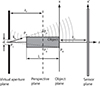Figure 1 Overview over the principle of hypercentric imaging using lensless digital-holography. The wave field is known across the camera plane x′ and can be reconstructed in the object plane x to yield an image of the object. However, for hypercentric imaging, we numerically apply a virtual aperture with diameter d. The aperture cuts out a part of the spherical wave of each object point and turns it into a ray-like wave field. Upon propagation into the perspective plane, this lets object points further away from the camera shift outwards across the image, as seen from PA and $P_A^{\text{'}}$. In contrast, object points closer to the camera, on the opposite side of the perspective plane, will appear shifted inwards. This behavior creates the hypercentric perspective.

In digital holography, imaging involves a numerical representation of the wavefield propagation process to calculate the wavefield $U_O\left(\vec{x}\right)$ directly in front of the object in a distance −z_O from the camera sensor$$U_O\left(\vec{x}\right)={\mathcal{P}}_{-z_O}\left\{U\left(\overrightarrow{x\text{'}}\right)\right\},$$(1)where ${\mathcal{P}}_z\{...\}$ denotes the propagation operator, which propagates a wave field by a distance z. One common example of such a propagation operator is realized in the angular spectrum method, where$${\mathcal{P}}_z\left\{U\left(\overrightarrow{x\text{'}}\right)\right\}={\mathcal{F}}^{-1}\left\{\mathcal{F}\left\{U\left(\overrightarrow{x\text{'}}\right)\right\}\cdot H_z\left(\vec{k}\right)\right\},$$(2)with the transfer function of free space propagation$$H_z\left(\vec{k}\right)=\exp \left(\mathrm{i}{k}_z\cdot z\right),$$(3)and the z-component k_z of the wave vector $\vec{k}$. The intensity $I_O\left(\vec{x}\right)=\left|U_O\right(\vec{x}){|}^2$ is the image of the object in focus. However, since we can freely select any distance z for the propagation in equation (1), holography provides volumetric imaging.

To understand how this can be used for hypercentric imaging, let us assume that the surface of the object can be described as a large number of point-like scattering sources. One of these scattering sources is indicated by P_A in Figure 1. The spherical wave emitted by P_A is stored as part of the digital hologram and will be propagated through space upon reconstruction, as indicated by the spherical wave fronts. We can now choose to reconstruct the wave field in the aperture plane and apply a virtual stop aperture. This is done by multiplying a window function W_d, which is 1 inside a disc of diameter d around the optical axis and 0 otherwise. If d is small enough, the aperture cuts out a segment of the spherical wave, which is strongly directed and travels mainly in the direction $-{\vec{k}}_A$. This effect of the aperture is crucial to hypercentric imaging. It turns an omnidirectional spherical wave into a directional, almost plane wave, similar to a ray.

After applying the aperture, the wave field is propagated back to a plane located in the center of the object, which we may refer to as the perspective plane. Due to its (now) almost ray-like nature, the wave field associated with P_A will let appear a point at the position ${\tilde{P}}_A$ in the perspective plane. Please note, how ${\tilde{P}}_A$ is laterally shifted outwards when comparing it with its true lateral position. In Figure 1 we also find the point P_B as a second example. If the same procedure is applied to it, it will appear at point ${\tilde{P}}_B$, shifted inwards across the perspective plane. This behavior is exactly what we expect from a hypercentric imaging system. Object parts far away from the observer, i.e. the camera sensor, appear larger than object parts close to it. The point P_C in the center of the aperture is the convergence point, where all ray-like wave fields intersect. Its position defines the characteristics of the perspective and the amount of hypercentricity.

With the simple geometry given in Figure 1, we can calculate the position ${\tilde{P}}_A$, depending on the true position P_A and z_P. For the sake of simplicity, we will describe P_A = (x_A, z_A) in two dimensions, with its position along the optical axis z_A and a single lateral coordinate x_A. Since the problem is fully separable, extension two three dimensions is trivial. With this in mind, and conveniently setting the origin to the convergence point P_C, the intercept theorem can be applied to find ${\tilde{x}}_A=\frac{x_A}{z_A}\cdot z_P$, or more generally, for any arbitrary point P = (x, z) in object space$$\tilde{x}=\frac{x}{z}·z_P.$$(4)

With equation (4), it is possible to calculate the depth dependent lateral shift of any object point due to the hypercentric perspective as$$\delta \tilde{x}=\tilde{x}-x=x\cdot \left(\frac{z_P}{z}-1\right).$$(5)

With the depth of the object L given, we can use equation (4) to calculate the perspective spread $\Delta \tilde{x}$, which we define as the maximum shift difference for object points with the same lateral position x, but at different axial positions along the object. The maximum shift difference is obtained for points at z = z_P − L/2 and z = z_P + L/2. Using equation (5) we find$$\Delta \tilde{x}\left(x\right)=\frac{x·z_P}{z_P-\frac{L}{2}}-\frac{x·z_P}{z_P+\frac{L}{2}}=\frac{x·z_P·L}{\left(z_P-\frac{L}{2}\right)\left(z_P+\frac{L}{2}\right)}\approx x\frac{L}{z_P},$$(6)where we have assumed that z_P is large against L/2 in the last step. The perspective spread can serve as a measure for the amount of hypercentricity, since it is zero for telecentricity and becomes even negative for entocentricity.

Finally, an important requirement to hypercentric imaging is, that the depth of field covers at least the depth of the object along the optical axis, which is denoted as L in Figure 1. This can be assured by selecting the diameter d of the virtual aperture properly. With air as medium (n ≈ 1) and small numerical apertures, the diffraction limited depth of field is given by$$z_D=\frac{\lambda \sqrt{(n^2-N{A}^2)}}{N{A}^2}\approx \frac{\lambda }{N{A}^2}.$$(7)

In this context, the numerical aperture for digital imaging into the perspective plane is defined by the diameter d and the imaging distance z_P, so that NA ≈ d/(2z_P). Inserting this into equation (7) and demanding z_D = L yields a useful rule to estimate the diameter of the aperture$$d=2z_P\sqrt{\frac{\lambda }{L}}.$$(8)

Please note, that in our case the depth of field z_D in equation (7) is oriented along the propagation direction of the ray-like wave fields. The propagation angles can become quite oblique, because of the large numerical aperture of the recording scheme. In most cases equation (8) still serves as a good estimate. However, for large propagation angles, exchanging z_D by its projection onto the opical axis z_D,⊥ is more accurate.

2.2 Holographic recording process

Figure 2 shows the recording configuration. The object illumination converges at P_C and has a particularly large numerical aperture, so that the sides of the specimen are illuminated as well. The reference wave is spherical, where the origin P_R has the same distance z_O from the camera sensor as the object’s surface, which is indicated by the surface point. This configuration resembles the scheme of Fourier holography [21, 22], even though object wave $U\left(\vec{x}\right)$ and reference wave $R\left(\vec{x}\right)$ need to be superposed by the 50:50 beam splitting plate to make them interfere. The camera sensor is a Sony IMX 661 with 13 408 × 9528 Pixel (127.7 MPix) and a pixel pitch of 3.45 μm. With an active surface area of 46 × 32 mm² (3.6″, it is significantly larger than the object, in order to collect light from the sides of the object. This yields a large numerical aperture in the observation path, which has to be matched by the reference wave. In our setup, this is realized by a microscope lens objective with NA = 0.28. However, fiber tips with large numerical aperture or pinholes could be used as well in order to make the setup more compact. The interference pattern recorded by the camera can be written as$$I\left(\vec{x}\right)=\left|U\right(\vec{x}){|}^2+|R\left(\vec{x}\right){|}^2+U^{\mathrm{*}}\left(\vec{x}\right)R\left(\vec{x}\right)+U\left(\vec{x}\right)R^{\mathrm{*}}\left(\vec{x}\right).$$(9)

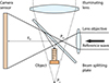Figure 2 Layout of the digital-holographic recording setup.

A piezo actuated mirror is placed in the reference path, to enable the introduction of phase shifts. The phase shifting process eliminates the twin image and the dc-term. For the hologram recording, a large number of phase shifting methods is available [21], where the methods differ in the achievable measurement uncertainty [22] and the stability against phase shifting errors [23]. We used 4 phase shifted digital holograms and a 4-frame 90° phase shifting algorithm [24], to yield the coherence function$$\mathrm{\Gamma }\left(\vec{x}\right)=U\left(\vec{x}\right)R^{\mathrm{*}}\left(\vec{x}\right).$$(10)

In our setup we have chosen a 50:50 beam splitting plate rather than a beam splitting cube. This allows to position the object closer to the camera and thus increases the NA of the recording geometry. Additionally, it has the advantage that spurious reflections from the sides of the glass cube are avoided. We also recommend inserting the beam splitting plate so that the 50% reflecting surface is oriented towards the object. With this, the ghost image from the back side is negligible. Additionally, we attached some absorbing black tape to the front side metal parts of the microscope objective in the reference path. This avoids spurious reflections from the metal housing due to the illumination.

2.3 Hypercentric rendering process

The hypercentric rendering process consists of two steps, which will be detailed below: The first step is a Fresnel reconstruction into the object plane. This is an efficient way to transfer the wavefield into object space while adjusting the scaling of the field of view to the size of the object, which is significantly smaller than the camera sensor. In the second step, we use the angular spectrum method to propagate the wave field into the aperture plane, apply the virtual aperture and then propagate the filtered wave field back to the perspective plane to finally yield a hypercentric image.

For the first step, we will have a look at the Fresnel diffraction integral for the (back) propagation of a wavefield in a distance −z_O, which, in our case, is the object plane: [25]$$U_O\left(\vec{x}\right)=\frac{\mathrm{i}}{\lambda z_O}\exp \left[\frac{-\mathrm{i}k|\vec{x}{|}^2}{2z_O}-\mathrm{i}k{z}_O\right]\cdot \mathcal{F}\left\{U\left(\overrightarrow{x\text{'}}\right)\cdot \exp \left(\frac{-\mathrm{i}k|\overrightarrow{x\text{'}}{|}^2}{2z_O}\right)\right\}\left(\frac{\vec{x}}{\lambda z_O}\right).$$(11)

The reference wave is a spherical wave with radius z_O, which can be approximated by a parabolic phase function$$R\left(\vec{x}\right)\approx \exp \left(\mathrm{i}k\frac{|\vec{x}{|}^2}{2z_O}\right).$$(12)

Comparing equation (11) with equation (10) and equation (12), we can rewrite equation (11) to$$U_O\left(\vec{x}\right)=\frac{\mathrm{i}}{\lambda z_O}\exp \left[\frac{-\mathrm{i}k|\vec{x}{|}^2}{2z_O}-\mathrm{i}k{z}_O\right]\cdot \mathcal{F}\left\{\mathrm{\Gamma }\left(\overrightarrow{x\mathrm{\prime }}\right)\right\}\left(\frac{\vec{x}}{\lambda z_O}\right).$$(13)

This shows, that with the origin of the reference wave chosen to z_O, a simple Fourier transform of the coherence function $\mathrm{\Gamma }\left(\vec{x}\right)$ provides a numerical representation of the object image. However, to retrieve phase and amplitude of the wavefield $U_O\left(\vec{x}\right)$, we have to fully calculate equation (13).

For the numerical implementation it is important to remember that the Fresnel propagation integral changes the scaling of the sampling grid. For a grid with (pixel) pitch p′ and (edge) size S′ in the sensor plane, we yield a new grid with pitch$$p=\frac{\lambda z_O}{S\mathrm{\prime }}$$(14)

and size S = λz_O/p′ in the object plane. This is a very convenient side effect of the Fresnel approach, because the hypercentric imaging scheme requires a large numerical aperture on the observation side. This means that z_O is comparably small, so that the size of the field of view S will typically be much smaller than the edge length S′ of the camera. The Fresnel propagation therefore adapts the field of view conveniently to the size of the object, which needs to be much smaller than the camera sensor as well.

For the second step, we can use equation (2) for the propagation and apply the virtual aperture W_d with diameter d in the aperture plane:$$\tilde{U}\left({\vec{x}}_P\right)={\mathcal{P}}_{z_P}\left\{{\mathcal{P}}_{-(z_P+L/2)}\left\{U_O\left(\vec{x}\right)\right\}\cdot W_d\left(\overrightarrow{x\mathrm{\prime }}\mathrm{\prime }\right)\right\},$$(15)

where ${\vec{x}}_P$ is a vector in the perspective plane. Using the angular spectrum method, the pixel pitch and the field of view do not change during the propagation operation, so that we can use the pitch p as found by equation (14) to determine the size of the aperture in the numerical implementation. Finally, the intensity $\tilde{I}\left({\vec{x}}_P\right)=\left|\tilde{U}\right({\vec{x}}_P){|}^2$ is the hypercentric image.

3 Experimental results

For the experimental implementation of our hypercentric imaging approach, we used the digital-holographic setup from Figure 2 with high NA illumination from the top. As an object we chose a stainless steel screw turned upside down, with a diameter of 3.9 ± 0.1 mm and a depth of L = 9.9 ± 0.1 mm (not including the screw head), as shown in Figure 3a. This object offers great dimensions in depth and diameter and the structured sides of the object with a thread pitch of 0.7 mm are good indicators for the depth of field and the level of hypercentricity. Another important factor is a sufficiently large object roughness to get enough light scattered onto the sensor.

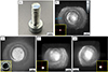Figure 3 a) The test object is a stainless steel screw turned upside down, with a diameter of 3.9 mm and a depth of L = 10 mm (not including the screw head). b) Digital-holographic hypercentric reconstruction of the object. The insert shows an image of the centered aperture with diameter d = 0.8 mm. The featured visible object depth is approx. 8 mm. Concerning the amount of hypercentricity we get a measured perspective spread of $\Delta {\tilde{x}}_m=0.43\pm 0.02\mathrm{ }\mathrm{mm}$, which is in very good accordance with the expected theoretical spread of $\Delta {\tilde{x}}_{\mathrm{theor}}=0.41\pm 0.03\mathrm{ }\mathrm{mm}$. c) From the same holographic data can also be calculated the conventional numerical reconstruction of the hologram. This yields a sharp image of the bottom surface of the screw. Because of the high-NA setup, the first screw threads are visible. (d, e) By shifting the lateral position of the virtual aperture, a sideways observation direction for the hypercentric imaging is selected. The insert shows an image of the laterally shifted aperture with d = 1.5 mm.

To attain the hypercentric image of the object from Figure 3b, we first calculate the object wave using equation (13) with a measured z_O = 9.3 ± 0.1 mm. Now we could directly obtain the conventional reconstruction of the recorded hologram, which yields a sharp image of the bottom surface of the screw, see Figure 3c. Because of the spiral structure of the screw and the angled illumination combined with the high-NA sensor, the first screw threads are also visible. But for the hypercentric imaging, we now choose a perspective plane, e.g. at L/2 in the middle of the object like in equation (15), and propagate from there to the aperture plane using the angular spectrum method from equation (2). Here, we apply a virtual aperture W_d with varying diameter d, depending on the desired lateral resolution and depth of field. This numerical application of the aperture marks the transition from the conventional imaging modality to the hypercentric one, all while relying on the same recorded hologram. Now, as described by equation (15), the backpropagation to the perspective plane finishes the hypercentric imaging process. In this case, all these steps are implemented numerically with z_P = 12 mm, d = 0.8 mm and the perspective plane 1 mm below the surface, yielding the hypercentric image of the object from Figure 3b. The hypercentricity is clearly visible in the high number of threads that are made visible by the hypercentric imaging effect, even from depths of approx. 8 mm below the surface.

Because of the small aperture needed to provide a depth of field that covers a majority of the object depth, the hypercentric imaging process generally comes with a drop in lateral resolution caused by the band limitation that is introduced with the (virtual) aperture. This is also the case for our digital-holographic approach, as can be seen in Figure 3b. Moreover, this band limitation brings about a filter for the direction of the light rays and establishes a predominant direction. Therefore, it comes with a side effect that makes the rough bottom surface of the screw look more specular. The overall degradation in image quality due to speckle noise is a common feature of holographic imaging in general. For further improvement of the image quality, speckle reduction methods from conventional holography can be applied. An overview of these de-noising strategies is given in [13, 26]. The level of hypercentricity $\Delta \tilde{x}\left(x\right)$ can be measured according to equation (6) by comparing the lateral coordinates in the perspective plane for two points. For the two positions $\tilde{x}$ marked in Figure 3b we get a measured perspective spread of $\Delta {\tilde{x}}_m=0.43\pm 0.02\mathrm{ }\mathrm{mm}$, which is in very good accordance with the expected theoretical spread of $\Delta {\tilde{x}}_{\mathrm{theor}}=0.41\pm 0.03\mathrm{ }\mathrm{mm}$.

The great advantage over lens-based hypercentricity is particularly demonstrated in the flexibility of the virtual aperture. In the axial dimension, z_P can be changed to adapt the amount of hypercentricity, as given by equation (6). In the lateral dimension, the purely numerical imaging process offers adaptation of the aperture diameter, but it even more offers the possibility to laterally shift the aperture inside the aperture plane and thereby select different observation directions, i.e. perspectives, from the same hologram. If we denote the lateral shift by Δr and consider the geometry introduced in Figure 1, it becomes clear that the effective observation angle towards the optical axis α is defined by tan(α) = Δr/z_P. Two examples for this are shown in Figures 3d and 3e for z_P = 9 mm, d = 1.5 mm and the perspective plane 4 mm below the surface, where the shift of the aperture results in a sideways perspective on one side of the object with an effective observation angle of α = 7.1° and α = 7.6°. Compared to Figure 3b, in Figure 3d and Figure 3e the effect of the larger aperture d is noticeable in the increased lateral resolution, traded against a smaller depth of field. Here, the perspective plane was changed afterwards by numerically refocusing to approx. the middle of the object at L/2 in order to get a sharp image of the side, even with the larger aperture. This ability to refocus to arbitrary perspective planes parallel to the sensor offers the possibility to extend the depth of field by numerical refocusing, although in this case the hypercentricity as given by equation (6), is changed with different z_P, which has to be considered. Consequently, in order to keep the hypercentricity constant the aperture plane would have to be adjusted accordingly for a constant z_P. In a lens-based system, this would need mechanical adjustment of the focus position by axially shifting the objective. However, for our lensless approach this can be implemented with no great effort, as an exact adaptation of the virtual aperture position is possible at any time.

For further demonstration of the lensless hypercentric imaging, a stainless steel spring with a diameter of 4.3 ± 0.1 mm, a depth of L = 26 ± 0.1 mm and a thread pitch of approx. 2 mm was used, as shown in Figure 4a. In this case, the hypercentric perspective is realized using a centered aperture with d = 1.5 mm and an aperture plane at distance z_P = 12 mm from the perspective plane, which was chosen 1 mm below the top surface. The result is shown in Figure 4b and features a visible object depth of approx. 4 mm. These results prove the feasibility of digital-holographic hypercentric reconstruction and open completely new opportunities for the implementation and application of the hypercentric imaging process.

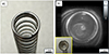Figure 4 a) The test object is a stainless steel spring with diameter of 4.3 ± 0.1 mm, a depth of L = 26 ± 0.1 mm and a thread pitch of approx. 2 mm. b) Digital-holographic hypercentric reconstruction of the object with an aperture of d = 1.5 mm, featuring a visible object depth of approx. 4 mm. The insert shows an image of the top of the object.

4 Conclusion

In this work, we have presented a novel approach for implementing hypercentric imaging on the basis of lensless digital holography. The imaging translates into the hypercentric imaging modality by applying a virtual aperture in the numerical reconstruction of the hologram. We developed a theoretical model describing the digital hypercentric imaging including all relevant parameters and tested it in experiment. Here, we demonstrated the feasibility of our new method by achieving highly resolved hypercentric perspectives on the object and showed how the imaging is affected by the positioning and sizing of the virtual aperture in axial and lateral dimensions. Moreover, we have shown that our theoretical model correctly predicts the level of hypercentricity, measured by the perspective spread, whereby a geometric model for this imaging modality is successfully established. It should be noted that our treatise is limited to the realm of scalar diffraction theory. Very large numerical apertures in the recording scheme and highly oblique propagation directions may require further extension towards vectorial optics.

The purpose and the main novelty of this work is the introduction of a lensless hypercentric imaging based on digital holography. Therefore, at the moment, the given examples mainly focus on qualitative imaging in order to introduce and demonstrate the lensless imaging functionality and to describe its main governing parameters. However, in future work this method can be expanded into all areas where hypercentric imaging is beneficial, especially in industrial inspection and in optical metrology. Embedded in the framework of lensless digital holography and its advantages like numerical refocusing and freely adaptable virtual apertures, the hypercentric imaging modality offers great potential for interferometric inspection applications.

Funding

This work was funded by the German Research Foundation (Deutsche Forschungsgemeinschaft, DFG) under the project: Hypercentric Imaging in Coherent Optical Metrology, “HyperCOMet” (Project number 430572965).

Conflicts of interest

There are no conflicts of interest.

Data availability statement

The underlying data is not publicly available at the time but can be provided by the authors upon reasonable request.

Author contribution statement

Conceptualization, C. Falldorf and B. Gutierrez; Specimen preparation, B. Gutierrez; Experimental measurements, B. Gutierrez and C. Falldorf; Evaluation and processing of experimental data, B. Gutierrez; Assessment of results, B. Gutierrez, C. Falldorf; Visualization, B. Gutierrez; Writing – Original Draft Preparation, C. Falldorf, B. Gutierrez, R. B. Bergmann; Supervision, R. B. Bergmann; All authors discussed the results and contributed to the final manuscript.

References

All Figures

Figure 1 Overview over the principle of hypercentric imaging using lensless digital-holography. The wave field is known across the camera plane x′ and can be reconstructed in the object plane x to yield an image of the object. However, for hypercentric imaging, we numerically apply a virtual aperture with diameter d. The aperture cuts out a part of the spherical wave of each object point and turns it into a ray-like wave field. Upon propagation into the perspective plane, this lets object points further away from the camera shift outwards across the image, as seen from PA and $P_A^{\text{'}}$. In contrast, object points closer to the camera, on the opposite side of the perspective plane, will appear shifted inwards. This behavior creates the hypercentric perspective.

In the text

	Figure 2 Layout of the digital-holographic recording setup.
In the text

Figure 3 a) The test object is a stainless steel screw turned upside down, with a diameter of 3.9 mm and a depth of L = 10 mm (not including the screw head). b) Digital-holographic hypercentric reconstruction of the object. The insert shows an image of the centered aperture with diameter d = 0.8 mm. The featured visible object depth is approx. 8 mm. Concerning the amount of hypercentricity we get a measured perspective spread of $\Delta {\tilde{x}}_m=0.43\pm 0.02\mathrm{ }\mathrm{mm}$, which is in very good accordance with the expected theoretical spread of $\Delta {\tilde{x}}_{\mathrm{theor}}=0.41\pm 0.03\mathrm{ }\mathrm{mm}$. c) From the same holographic data can also be calculated the conventional numerical reconstruction of the hologram. This yields a sharp image of the bottom surface of the screw. Because of the high-NA setup, the first screw threads are visible. (d, e) By shifting the lateral position of the virtual aperture, a sideways observation direction for the hypercentric imaging is selected. The insert shows an image of the laterally shifted aperture with d = 1.5 mm.

In the text

	Figure 4 a) The test object is a stainless steel spring with diameter of 4.3 ± 0.1 mm, a depth of L = 26 ± 0.1 mm and a thread pitch of approx. 2 mm. b) Digital-holographic hypercentric reconstruction of the object with an aperture of d = 1.5 mm, featuring a visible object depth of approx. 4 mm. The insert shows an image of the top of the object.
In the text

References

- Ulrich M, Steger C, A camera model for cameras with hypercentric lenses and some example applications, Mach. Vision Appl. 30, 1013–1028. [Google Scholar]
- Schnars U, Falldorf C, Watson J, Jüptner W, Computational wavefield sensing, in Digital holography and wavefront sensing: principles, techniques and applications (2015), pp. 141–184. [Google Scholar]
- Ozcan A, McLeod E, Lensless imaging and sensing, Ann Rev. Biomed. Eng. 18, 77–102 (2016). [Google Scholar]
- Boominathan V, Robinson JT, Waller L, Veeraraghavan A, Recent advances in lensless imaging, Optica 9, 1–16 (2022). [CrossRef] [PubMed] [Google Scholar]
- Falldorf C, Müller AF, Pazos BG-C, Bich JA, Bergmann RB, Current progress in lensless holographic microscopy, 3D Imag. Visual. Display (SPIE, 2025) 13465, 19–26 (2025). [Google Scholar]
- Moon I, Javidi B, Volumetric three-dimensional recognition of biological microorganisms using multivariate statistical method and digital holography, J. Biomed. Opt. 11, 064004–064004 (2006). [Google Scholar]
- Kim J, Go T, Lee SJ, Volumetric monitoring of airborne particulate matter concentration using smartphone-based digital holographic microscopy and deep learning, J. Hazard. Mater. 418, 126351 (2021). [Google Scholar]
- Pazos BG-C, Falldorf C, Bergmann RB, Lensless sideways imaging with digital holography for in-line process monitoring in additive manufacturing, in Multimodal Sensing and Artificial Intelligence for Sustainable Future 13570, 196–202 (2025). [Google Scholar]
- Colomb T, et al., (2010) Extended depth-of-focus by digital holographic microscopy, Opt. Lett. 35, 1840–1842. [Google Scholar]
- Pedrini G, Schedin S, Tiziani HJ, Aberration compensation in digital holographic reconstruction of microscopic objects, J. Modern Opt. 48, 1035–1041 (2001). [Google Scholar]
- Gao P, Yuan C, Resolution enhancement of digital holographic microscopy via synthetic aperture: a review, Light Adv. Manuf. 3, 105–120 (2022). [Google Scholar]
- Falldorf C, Luepke SH-V, Von Kopylow C, Bergmann RB, Reduction of speckle noise in multiwavelength contouring, Appl. Opt. 51, 8211–8215 (2012). [Google Scholar]
- Bianco V, et al., Quasi noise-free digital holography, Light Sci. Appl. 5, e16142 (2016). [Google Scholar]
- Schnars U, Falldorf C, Parallax limitations in digital holography: a phase space approach, Light Adv. Manuf. 3, 400–407 (2022). [Google Scholar]
- Min J, et al., Simple and fast spectral domain algorithm for quantitative phase imaging of living cells with digital holographic microscopy, Opt. Lett. 42, 227–230 (2017). [Google Scholar]
- Wu Y, Ozcan A, Lensless digital holographic microscopy and its applications in biomedicine and environmental monitoring, Methods 136, 4–16 (2018). [Google Scholar]
- Kumar M, et al., Single-shot common-path off-axis digital holography: applications in bioimaging and optical metrology, Appl. Opt. 60, A195–A204 (2020). [Google Scholar]
- Osten W, Ferraro P, Optical Inspection of Microsystems , Second Edition, (CRC Press, 2019), pp. 405–484. [Google Scholar]
- Fratz M, Seyler T, Bertz A, Carl D, Digital holography in production: an overview, Light Adv. Manuf 2, 283–295 (2021). [Google Scholar]
- Falldorf C, Thiemicke F, Müller AF, Agour M, Bergmann RB, Flash-profilometry: fullfield lensless acquisition of spectral holograms for coherence scanning profilometry, Opt. Expr. 31, 27494–27507 (2023). [Google Scholar]
- Kim S, Jeon J, Kim Y, Sugita N, Mitsuishi M, Design and assessment of phase-shifting algorithms in optical interferometer, Int. J. Precis. Eng. Man-GT 10, 611–634 (2023). [Google Scholar]
- Hack E, Burke J, Invited review article: measurement uncertainty of linear phase-stepping algorithms, Rev. Sci. Instrum. 82, 061101 (2011). [Google Scholar]
- Guo C-S, Zhang L, Wang H-T, Liao J, Zhu Y, Phase-shifting error and its elimination in phase-shifting digital holography, Opt. Lett. 27, 1687–1689 (2002). [NASA ADS] [CrossRef] [Google Scholar]
- Carré P, Installation et utilisation du comparateur photoélectrique et in terférentiel du Bureau International des Poids et Mesures, Metrologia 2, 13 (1966). [Google Scholar]
- Müller AF, Bergmann RB, Falldorf C, High resolution lensless microscopy based on Fresnel propagation, Opt. Eng. 63, 111805 (2024). [Google Scholar]
- Bianco V, et al. Strategies for reducing speckle noise in digital holography. Light Sci. Appl. 7, 48 (2018). [Google Scholar]