| Issue |
J. Eur. Opt. Society-Rapid Publ.
Volume 21, Number 2, 2025
|
|
|---|---|---|
| Article Number | 43 | |
| Number of page(s) | 13 | |
| DOI | https://doi.org/10.1051/jeos/2025038 | |
| Published online | 26 September 2025 | |
Research Article
Dual-window transformer framework with pyramid structure and constrained self-attention for hyperspectral anomaly detection
Shijiazhuang Campus, Army Engineering University of PLA, Shijiazhuang, Hebei 050000, PR China
* Corresponding author: This email address is being protected from spambots. You need JavaScript enabled to view it.
Received:
15
July
2025
Accepted:
3
September
2025
Abstract
Hyperspectral anomaly detection (HAD) is widely used in various fields including military, agriculture, mining, and food safety inspection. However, the absence of prior information on targets poses significant challenges to feature extraction and anomaly identification. To address this issue, this paper proposes a novel dual-window transformer framework integrated with a pyramid structure and constrained self-attention mechanism, which effectively leverages both local and global spectral information for anomaly detection. The dual-window transformer is designed to extract deep spectral features by capturing discriminative patterns between central pixels and their surrounding background. Simultaneously, the constrained self-attention module incorporates global contextual information into the feature representation. Furthermore, a stepwise downsampling pyramid architecture is introduced to reduce the sensitivity of the model to dual-window size selection while facilitating the propagation of global information from higher to lower layers. Extensive hyperparameter analysis and comparative experiments demonstrate the robustness and superiority of the proposed framework. The source code is publicly available at: https://github.com/aosilu/DWT-P-CSA-HAD.
Key words: Anomaly detection / Transformer / Pyramid structure / Hyperspectral image
© The Author(s), published by EDP Sciences, 2025
 This is an Open Access article distributed under the terms of the Creative Commons Attribution License (https://creativecommons.org/licenses/by/4.0), which permits unrestricted use, distribution, and reproduction in any medium, provided the original work is properly cited.
1 Introduction
Hyperspectral imagery constitutes three-dimensional data characterized by high spectral resolution and rich spectral information, facilitating precise pixel-level classification. Within such imagery, anomalous targets typically occupy a minimal number of pixels and exhibit spectra markedly distinct from their surrounding background [1–5]. Hyperspectral anomaly detection (HAD) identifies anomalous pixels without prior knowledge of target or background spectral signatures [6–8].
The research on hyperspectral anomaly detection can be divided into traditional and deep learning methods. The Reed-Xiaoli (RX) algorithm [9] is a classic statistical approach among traditional methods; it calculates the anomaly level of pixels by assuming that the background follows a multivariate normal distribution. The local variant of the RX algorithm [10] uses a dual-window to select the background instead of using the entire image, calculating the local anomaly level for each pixel. A weighted method is also used in the RX algorithm [11], which assigns low weights to abnormal samples and can better estimate the background distribution. The two-step generalized likelihood ratio test (2S-GLRT) [12] utilizes design criteria based on the generalized likelihood ratio test and its two-step modification to reduce computational complexity while improving detector performance. The development of compressive sensing theory has led to the use of reconstruction-based methods in HAD. The sparse representation (SR) model [13] reconstructs all pixels using an overcomplete dictionary, while the residuals represent the degree of pixel anomalies. Collaborative representation (CR) [14] is one of the commonly used reconstruction methods, which allows all atoms in the dictionary to participate in linear representation and is a pixel-by-pixel detection method. Low-rank representation (LRR) [15] divides data into sparse backgrounds and anomalies, focusing on describing the global structure of hyperspectral images. The attribute and edge-preserving filtering-based anomaly detection (AED) method [16] utilizes morphological filtering and support vector machines to achieve anomaly detection, integrating spatial and spectral information. With the deepening of research, deep learning-based HAD technology is gradually receiving attention, and its detection framework is divided into supervised and unsupervised approaches. Li et al. [17] proposed a supervised anomaly detection framework based on transferred deep CNN, which trains using differential pixel pairs formed by different categories of ground objects in reference images, with the difference between the central pixel and surrounding pixels as the anomaly level of the central pixel. Stacked autoencoder (SAE) [18] is a typical unsupervised deep learning network that reconstructs hyperspectral images through an encoder-decoder structure. Abnormal targets cannot be accurately identified by restoring their spectra. The Auto-AD [19] method uses full convolutional layers to construct autoencoders, which can suppress abnormal reconstruction. Fan et al. [20] proposed robust graph autoencoders (RGAE) that preserve the geometric structure between training samples and are robust to noise and anomalies during the training process.
Recent years have witnessed increasing adoption of transformer models in HAD for their potent global information extraction. Liu et al. [21] introduced BiGSeT, employing a binary mask-guided separation training strategy to address the identical mapping problem (IMP) via latent binary mask-based loss, effectively suppressing anomalies during background reconstruction. Ma et al. [22] developed a coarse-to-fine multiview anomaly coupling network integrating axial attention for global features and residual CNNs for fine-grained local characteristics, enhancing detection accuracy. Wu et al. [23] proposed a 3D-Transformer network leveraging spatial pixel correlations and spectral band similarities to reduce false alarms in background reconstruction. Xiao et al. [24] devised S2DWMTrans, aggregating global background perspectives while suppressing anomalies via dual-window neighboring pixels. Lian et al. [25] presented GT-HAD, a gated Transformer exploiting spatial-spectral similarity with dual-branch modeling and adaptive gating units. Wang et al. [26] established a self-supervised method using finite spatialwise attention (FSA) to mine background spectral clustering structures. Zhang et al. [27] created a differential network combining local punctured neighborhood extraction with detail and Transformer attention mechanisms. Li et al. [28] proposed an explicit background endmember learning framework (EBEL), which learned background endmember features using a cross-attention mechanism and represented hyperspectral image features through a cascaded cross-attention-based module, thereby improving anomaly detection performance. He et al. [29] proposed a convolutional Transformer-inspired autoencoder (CTA), which combined convolutional and Transformer architectures to capture both local and global features, thereby improving anomaly detection performance. Liu et al. [30] proposed SSHAD, an adaptive dual-domain learning method for HAD with state-space models. This method combined a spatial-wise selected state space module (SSSM) and a spectral-wise frequency division self-attention module (FDSM) to capture both spatial sparsity and inter-spectral similarity in hyperspectral images, thereby improving detection performance. Sun et al. [31] introduced CSSBR, a contrastive self-supervised learning-based background reconstruction method, which employed a pixel- and patch-level masking strategy and a dual-attention network (DAN) encoder to learn universal background representations without labeled samples. Guo et al. [32] proposed SSCMAE, a spatial-spectral cross-guided masked autoencoder, which used a guided mask based on spectral differences to suppress anomaly reconstruction and enhance background reconstruction accuracy. Additional contributions include: Spectrum Difference Enhanced Network (SDENet) [33] amplifying spectral discrepancies through variational mapping and Transformer; Transformer-Based Autoencoder Framework (TAEF) [34] modeling nonlinear mixing via autoencoder-Transformer integration; TGFA-AD [35] reconstructing abundance matrices with Transformer encoders and fractional convolution; adversarial refinement-based inpainting methods [36]; and the “train-once” anomaly enhancement network [37]. These studies collectively demonstrate the significant advancements in HAD enabled by deep learning and Transformer architectures. Each method emphasizes different aspects of feature extraction, background reconstruction, and anomaly suppression, contributing to the ongoing development of this field [38, 39].
With the rapid development of detector technology and UAV technology, handheld and UAV imaging spectrometers have been widely used, resulting in a large number of handheld/UAV spectrometer data [40]. This kind of hyperspectral image has the characteristics of “double high resolution”, that is, high spatial resolution and high spectral resolution, and the acquisition angle is variable. Data are often used immediately without various corrections, resulting in greater spectral variability and difficulties in extracting deep spectral features [41]. Due to the close data collection distance and high spatial resolution, the spatial distribution of the image is complex and large-scale continuous features may no longer exist (for example, leaves, branches, tree trunks, and grass may alternate in the space in the jungle). We hope to observe the performance of the proposed method on this type of data, so the data in this article are all private near ground data taken from near ground sources [42].
We propose a dual-window transformer framework with pyramid structure and constrained self-attention for anomaly detection in hyperspectral images. This framework only learns the differences in pixels between the center pixel and the dual-window. The selection of dual-window size is an unavoidable issue for all “window methods”. We construct an image pyramid by spatially sampling hyperspectral images, which are preprocessed and input layer by layer into the constrained self-attention transformer module. The output results are spatially upsampled as “intrinsic constraints” and fed back to the next layer’s constrained self-attention module along with “external constraints”, greatly reducing the impact of window size on detection results. External constraints are generated by SAE, which can enhance the robustness of the overall framework and provide information for the constrained self-attention transformer module at the first layer runtime.
The main contributions of the method proposed in this article can be summarized as follows:
-
We propose a dual-window transformer framework with pyramid structure and constrained self-attention. The proposed framework utilizes a pyramid structure to weaken the impact of window size on model performance.
-
The dual-window model can extract local information from hyperspectral images and fuse it with the global information feedback from the pyramid structure to the upper constrained self-attention transformer module, effectively detecting abnormal targets in hyperspectral images.
-
We conducted experimental verification using real hyperspectral images and compared them with state-of-the-art methods, ultimately proving the effectiveness of our proposed method.
2 Preliminary
2.1 Multi-head attention
The Transformer is a deep learning model proposed by Vaswani et al. [43] for natural language processing; it processes all elements in a sequence in parallel and can efficiently and quickly capture long-term dependencies in text. The Vision Transformer (ViT) uses the encoder module from the Transformer architecture for image classification tasks by segmenting images into patches and flattening them. This approach transforms the image recognition problem into a “sequence-to-sequence” problem [44]. The core of the Transformer encoder is the multi-head attention (MSA) mechanism, where each self-attention (SA) corresponds to a set of matrices Wq, Wk, and Wv, which are multiplied by the input X of SA to obtain the query Q, key K, and value V as follows: (1)
(1)
The corresponding output of SA is: (2)
(2)
The product of Q and K
T represents similarity, while V can be seen as a vector of a single input feature. Figure 1 illustrates the computation of multi-head attention as implemented in the actual code. It consists of multiple self-attention mechanisms. The input X is split into segments, and the corresponding self-attention is computed based on equations (1) and (2). These are then concatenated to obtain Z, which satisfies the following equation: (3)where h is the number of self-attention groups.
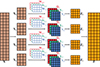 |
Fig. 1 The calculation process of multi-head attention. |
2.2 Stacked autoencoder
The Autoencoder is an unsupervised neural network model designed to learn deep features of data and reconstruct the input. Essentially, it is a three-layer neural network comprising an input layer, a hidden layer, and a reconstruction layer [45]. Figure 2 shows the structure of a stacked Autoencoder, which is a symmetric multi-layer neural network formed by stacking multiple Autoencoders. The output of the lth layer in the stacked Autoencoder is:![Mathematical equation: $$ {\mathbf{y}}^{(l)}=f\left[{\mathbf{W}}^{(l)}{\mathbf{y}}^{\left(l-1\right)}+{\mathbf{b}}^{(l)}\right]. $$](/articles/jeos/full_html/2025/02/jeos20250047/jeos20250047-eq4.gif) (4)
(4)
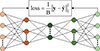 |
Fig. 2 Diagram of stacked autoencoder (SAE). |
3 Proposed method
In this section, we specifically introduce the proposed dual-window transformer framework with pyramid structure and Constrained self-attention. Figure 3 shows the framework of the proposed method, a pyramid structure where the final result of each layer’s operation provides feedback for the next layer. The hyperspectral images of each scale in the pyramid are entered into Dual window Preprocessing and Constrained self-attention transformer module (CSATM) in order of scale. The framework’s core is the CSATM, whose weight of self-attention is Constrained by the upper layer of the pyramid. The framework consists of four parts:
-
Pyramid construction: Hyperspectral images are downsampled step by step spatially and input into subsequent modules. After completing all subsequent modules of a certain scale hyperspectral image, input the next scale hyperspectral image.
-
Dual-window preprocessing: The pixel-by-pixel moving dual-windows extract the hyperspectral image into a set of “center pixels – pixels within the dual-window”, and process the set into a form that can be received by CSATM. The center pixel and background pixel of the dual window at a certain position form a training sample.
-
CSATM: The core part of the framework is to learn spectral depth differences and provide pixel-level anomaly score maps.
-
Constraints generation module (CGM): Integrate intrinsic constraints and external constraints into self-attention constraints, and input into CSATM.
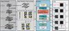 |
Fig. 3 Framework of the proposed method. |
3.1 Image pyramid
Input the hyperspectral image  and perform progressive spatial downsampling at a ratio of 1/2 to obtain Y
(0), Y
(2), and Y
(3). Y
(3) will enter the subsequent modules as the input for the first layer, and after the intrinsic constraints and external constraints of the first layer are fed back to CSATM, Y
(2) will be inputted. The same operation is used for Y
(1) and Y
(0).
and perform progressive spatial downsampling at a ratio of 1/2 to obtain Y
(0), Y
(2), and Y
(3). Y
(3) will enter the subsequent modules as the input for the first layer, and after the intrinsic constraints and external constraints of the first layer are fed back to CSATM, Y
(2) will be inputted. The same operation is used for Y
(1) and Y
(0).
3.2 Dual-window preprocessing
Take the input Y
(0) of the fourth layer as an example. Y
(0) performs boundary padding to ensure normal processing of boundaries by the dual-window and is then extracted as a set of “center pixels – dual-window inner pixels” by the dual-window with outer window size winout and inner window size winin. The set is represented as: (5)where
  , M = H × W.
The purpose of the overall framework is to learn the level of difference between the central pixel and the surrounding background, and the required residuals are obtained as follows: (6)
(6)
In this section, the hyperspectral image Y (0) ∈ ℝ H × W × B is converted into ε ∈ ℝ M × N × B , which can be processed by CSATM.
3.2 CSATM
The differential data ε ∈ ℝ
M × N × B
is encoded as deep features in this module, and the anomaly score is finally obtained. The fully connected layer in the Embedded module performs a linear transformation on ε and adds positional information. The encoded vector is passed through a constrained transformer encoder and finally processed by Mean and MLP to obtain the anomaly score S. The forward process is as follows: (7)
(7)
Where CMSA(x) = concat(CSA1, CSA2, …, CSA
h
). The new weights obtained by adding constraints to self-attention weights are as follows:![Mathematical equation: $$ \mathbf{CSA}=\mathrm{Softmax}\left[\mathbf{Q}{\mathbf{K}}^T\mathrm{Norm}\left({\mathbf{\gamma \gamma }}^T\right)\right]\mathbf{V}, $$](/articles/jeos/full_html/2025/02/jeos20250047/jeos20250047-eq10.gif) (8)
(8)
 (9)
(9)
 (10)where
  is the value corresponding to the central pixel in the intrinsic constraints;
  is the value corresponding to pixels within the dual-window in the intrinsic constraints;
  is the value corresponding to the central pixel in the external constraints;
  is the value corresponding to the pixels within the double window in the external constraints. Figure 4 shows the positions of
  and
and  , with the same distribution of external constraints.
  is the central pixel to be tested, and
  is the surrounding background pixel.
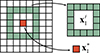 |
Fig. 4 Diagram of intrinsic constraints. |
3.4 GCM
The results of each layer will be input into CSATM as intrinsic constraints. The training of the first layer does not provide intrinsic constraints for the previous layer. We stagger the number of layers of intrinsic constraints and external constraints and provide the first layer of external constraints to the first layer of CSATM. External constraints obtained from SAE represent the addition of global information, which can make the model more robust. Algorithm 1 briefly describes the acquisition of additional constraints, taking Y(0) as an example.
1. Input 
2. TRAIN
for i=1:(H×W)
 loss.backward
3. TEST
for i=1:(H×W)
![Mathematical equation: $ {\mathbf{r}}_i^{(0)}=[{\mathbf{y}}_i^{(0)}-\mathrm{SAE}({\mathbf{y}}_i^{(0)})]\in {\mathbf{R}}^{(\mathbf{0})}$](/articles/jeos/full_html/2025/02/jeos20250047/jeos20250047-eq29.gif)
![Mathematical equation: $ \mathbf{\mu }=\mathrm{mean}\left[{\mathbf{R}}^{\left(\mathbf{0}\right)}\right],\mathbf{K}=\mathrm{cov}[{\mathbf{R}}^{(\mathbf{0})}]$](/articles/jeos/full_html/2025/02/jeos20250047/jeos20250047-eq30.gif)
for i=1:(H×W)
reshape S(0)
4. Output results S(0) ∈ ℝH × W
The hyperspectral image is input into SAE, but the anomaly cannot be well reconstructed by the network due to its unique characteristics. Therefore, the residual between the original image and the reconstructed image can reflect the location of the anomaly. Apply the RX algorithm on residuals to obtain external constraints. The result  generated by the first layer is spatially upsampled twice to obtain the first intrinsic constraint, which is fed back to CSATM along with the second external constraint
  . When running to the last layer, the weighted average of the intrinsic constraint
  and the last external constraint
  is used as the final result.
4 Experimental results and analysis
4.1 Datasets and experimental setup
This article uses five real hyperspectral data for experiments, and their pseudocolor images and the corresponding ground-truth maps are shown in Figure 5. The spectral component of the hyperspectral imager is Acousto-Optic Tunable Filter (AOTF), and we have set the wavelength range to 449–801 nm, which includes 89 bands with band intervals of 4 nm.
-
Meadow: The image resolution is 1000 × 400, with fake turf-A placed as the abnormal target, and the background includes building walls and lawns.
-
Holly: The image resolution is 600 × 496, with fake turf-B placed as the abnormal target, and the background includes holly flower beds and architectural shadows. Meadow and Holly were both filmed on May 26, 2022, with geographic coordinates (38°27′W, 114°30′E) and a ground spatial resolution of approximately 8.4 mm, both of which belong to typical urban near ground scenes.
-
Cement Street: The image resolution is 500 × 300. Filmed on April 6, 2024, with geographic coordinates (38°27′W, 114°30′E) and a ground spatial resolution of 1.5 mm, it belongs to a cement road background and targets two alloy aircraft models.
-
Jungle-I and Jungle-II: Filmed on April 6, 2024, with geographic coordinates (38°27′W, 114°30′E) and a ground spatial resolution of 3.3 mm, all of which belong to a close-range jungle background, and the image resolution is 1000 × 1000. Different types of fake turf-C and fake turf-D were placed in Jungle-I and Jungle-II. Meadow serves as the training set for the entire framework.
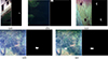 |
Fig. 5 Pseudocolor images (left) and the corresponding ground-truth maps (right) of five real hyperspectral datasets. (a) Meadow; (b) Holly; (c) Cement Street; (d) Jungle-I; (e) Jungle-II. |
All experiments were implemented on the Ubuntu system using PyTorch 1.8 and Python 3.8, with two GeForce GRX 2080 GPUs included. Table 1 shows the model parameter settings for the Transformer module and SAE in the proposed framework. Meadow will serve as the training set for the framework.
CSATM and SAE parameter settings.
4.2 Evaluation metrics
There are objective and subjective analyses of the results of HAD. The subjective analysis mainly involves decision-makers combining ground-truth maps to visually analyze the detection results. The most commonly used methods in objective analysis are receiver operating characteristics (ROC) and area under the curve (AUC). The ROC curve establishes a correlation between the probability of false alarm (PFA) and the probability of detection (PD), which is based on a common threshold τ. The traditional two-dimensional ROC curve is essentially composed of τ-PFA relationship curve and τ-PD relationship curve. The definitions of PD and PFA are as follows: (11)where Nd is the number of real target pixels detected, which is the number of pixels that belong to the target and are considered the target by the detector, Nt represents the total number of target pixels in the image. Nf represents the number of detected false alarm pixels, which belong to the background but are considered targets by the detector. Nb represents the total number of background pixels in the image.
AUC quantitatively describes the degree of deviation of the ROC curve to the upper left, which is the area formed by the ROC curve surrounded by the horizontal axis. The values are as follows: (12)
(12)
The greater the offset of the ROC curve to the upper left, the larger the area below the curve line, and the larger the AUC, indicating better detection performance. The flatter the ROC curve, the smaller the area below the curve, and the smaller the AUC, the worse the detection effect.
4.3 Hyperparameter analysis
The framework proposed in this article has some pre-set hyperparameters. This section will analyze the impact of hyperparameters on the framework through ablation experiments and select appropriate hyperparameters to achieve optimal detection performance.
4.3.1 The impact of dual-window size on the model
Set the range of the outer window size winout to [3, 5, 7] and the range of the inner window size winin to [1, 3, 5]. Different winin and winout will be combined into six sets of dual-window parameters. In this section of the experiment, the heads (number of self-attention) of CASTM are set to 1, and the depth (number of encoder blocks) is set to 5. The experiment will be conducted on the remaining four datasets, with AUC values as the evaluation metric. Table 2 shows the detection results for different dual-window sizes. On each dataset, the difference between the highest and lowest AUC is less than 0.01, indicating that changes in the dual-window parameter group have a very small impact on the detection performance of the model. Based on this conclusion, when winout is fixed, the influence of the thickness (th = winout − winin − 1) of the double window on the detection results can be ignored. Figure 6 shows the detection results for each dataset at th = 1 for different dual-window. Holly and Jungle-I showed mild performance, while Cement Street and Jungle-II changed when the dual-window reached (9, 11), but the overall change was not significant. We take the dual-window parameter group (9, 11) with the highest average AUC value from the four datasets as the optimal parameter.
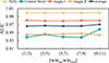 |
Fig. 6 AUC under different dual-windows when heads = 1. |
AUC under different dual-window.
4.3.2 The impact of the number of heads and depths on the model
The number of heads affects the model’s ability to capture differences across the entire spectral band, and an appropriate number of heads should be considered. The depth of the model represents the number of encoder blocks, which affects the model’s ability to extract features based on the difference between pixels in the dual-window and the center pixel. In this section of the experiment, we set the dual-windows to (9, 11). Figure 7 shows the detection results of each dataset under different numbers of heads at depth = 5. The experiment shows that the model performs best when heads = 6. Figure 8 shows the detection results of each dataset at different depths when heads = 6, with the best performance achieved at depth = 5.
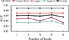 |
Fig. 7 AUC under different numbers of heads when depth = 5. |
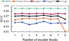 |
Fig. 8 AUC under different depths when heads = 6. |
In the end, we chose heads = 6, depth = 5, and (winin, winout) = (9, 11) as the optimal hyperparameter group for the framework.
4.4 Ablation experiment
This section will discuss the role and effectiveness of the proposed constrained self attention transformer module in the framework. The experiment will test the anomaly detection performance of traditional self attention and constrained self attention on various datasets. Table 3 shows the results of the experiment. Although CSATM performs slightly worse than MSA on the Cement Street dataset, their detection results have AUC values close to 1, and the difference can be ignored. More attention should be paid to the performance on the other three datasets. The performance of CSATM on Holly, Jungle-I, and Jungle-II datasets has significantly improved compared to MSA, indicating that CSATM has stronger feature extraction ability and detection performance. The main reason for the excellent performance of CSATM is that it obtains additional information based on MSA, including local anomaly information at the downsampling scale and global anomaly information provided by SAE. These additional information enable CSATM to adaptively adjust its self-attention weights and improve the performance of the model.
AUC value of detection results using CSATM and MSA frameworks.
4.5 Comparative experiment
In order to effectively analyze and evaluate our proposed detection framework, the comparison methods we use include:
-
RX [4]: Assumes background adherence to Gaussian distribution. Estimates the probability density function via background covariance and mean vectors, defining anomaly level as test pixel deviation from background statistical distribution.
-
2S-GLRT [7]: Adaptive detector for Gaussian backgrounds with unknown covariance matrices, implementing generalized likelihood ratio testing.
-
CRD [9]: Sparse representation-based detection method constructing dictionaries to represent targets/backgrounds. Represents target signals as linear combinations of dictionary atoms, separating targets/backgrounds through sparse coefficient optimization.
-
RGAE [15]: Graph-regularized autoencoder framework maintaining geometric sample structures and demonstrating noise/anomaly robustness during training.
-
Auto-AD [14]: Skip-connected fully convolutional autoencoder employing adaptive weighted loss to suppress abnormal pixel contributions during reconstruction.
-
CTA [24]: Integrates K-means clustering (extracting pseudo-background/anomalous samples) with convolutional Transformer autoencoders. Combines convolutional layers and multi-head attention to capture local-global features, enhancing anomaly-background separability.
-
GT-HAD [20]: Leverages spatial-spectral similarity during reconstruction with du-al-branch modeling (background/anomaly features) under content similarity constraints. Incorporates adaptive gating units via Content Matching Method (CMM) for branch activation control.
-
TAEF [30]: Embeds Extended Multilinear Mixture Model (EMLM) in decoder while utilizing Transformer-based encoder. Effectively reconstructs HSI backgrounds and characterizes high-order nonlinear mixing phenomena.
The setting with hyperparameters in the comparison method is:
-
2S-GLRT: The size of the dual-window (winin, winout) = (5, 7).
-
CRD: The size of the dual-window (winin, winout) = (3, 11), Lagrange Multiplier λ = 0.1.
-
RGAE: Tradeoff Parameter λ = 10-2, Number of Superpixels S = 150, Dimension of Hidden Layer n_hi d = 20.
Figures 9–12 shows the detection results of each method on the Holly, Cement Street, Jungle-I, and Jungle-II datasets. From the overall detection results, traditional detection methods (RX, 2S-GLRT, and CRD) have weak detection performance, and their main characteristics are: 1) low target anomaly scores; 2) a large number of target pixels are missed and scattered; 3) a large number of false alarms in the detection results of the Cement Street dataset. The reason for these phenomena is that hyperspectral images captured near the ground have strong spectral uncertainty, and the phenomenon of “same substance but different spectrum, same spectral foreign objects” is more obvious. Traditional detection methods cannot extract deep spectral features, which can easily lead to missed detections and false alarms. The detection performance of RGAE, Auto-AD, GT-HAD, and TAEF is basically the same, but the detection rate of Jungle-I and Jungle-II data sets is not high. These models are all based on reconstruction based deep learning methods. The background of the Holly and Cement Street datasets is relatively simple, and these methods can effectively reconstruct the background to distinguish anomalous targets. The backgrounds of the Jungle-I and Jungle-II datasets are relatively complex, and the performance of reconstruction based methods on both datasets has significantly decreased. The detection results of CTA are not ideal, except for detecting edges in the Cement Street dataset, no targets are detected in the other three datasets. The training sample quality and model performance of CTA depend on its clustering-based module. The hyperspectral dataset we provide has a large spatial size and contains a large number of spectral training samples. The clustering-based module cannot effectively partition the anomaly and background sets, resulting in rapid model degradation. The proposed method has good integrity in detecting targets in four datasets, and its anomaly score is high, but there are some false alarms in the detection results. Figure 13 shows the ROC curves and log scale ROC curve of the detection results of each method on the Holly, Cement Street, Jungle-I, and Jungle-II datasets. 2S-GLRT has little detection effect on near-ground datasets. CTA is very accurate in distinguishing the background, but there are also issues with undetectable or incomplete detection of targets. Our proposed method performs the best overall, but its performance on Cement Streets is not as good as RGAE, Auto-AD, GT-HAD, and TAEF. Table 4 shows the AUC values of the ROC curves for the detection results of each method on the Holly, Cement Street, Jungle-I, and Jungle-II datasets. Holly and Cement Street have relatively simple backgrounds and generally perform well compared to the methods used, while Jungle-I and Jungle-II are close-range jungle backgrounds with complex backgrounds, resulting in a decrease in their detection performance. Our proposed method has the highest average AUC, but the performance varies on different datasets. Jungle-I and Jungle-II have the same background, but the proposed method has slightly different detection performance. The SAE in the proposed method is based on a reconstructed model, which adjusts the self attention weights together with the global anomaly information provided by the upper layer of the pyramid, resulting in better model performance than the reconstruction method. The experiments in this section have effectively demonstrated the superiority of the proposed method.
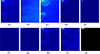 |
Fig. 9 The detection results of different methods on the dataset (Holly). (a) RX; (b) 2S-GLRT; (c) CRD; (d) RGAE; (e) Auto-AD; (f) CTA; (g) GT-HAD; (h) TAEF; (i) Proposed method; (j) Ground-truth maps. |
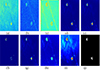 |
Fig. 10 The detection results of different methods on the dataset (Cement Street). (a) RX; (b) 2S-GLRT; (c) CRD; (d) RGAE; (e) Auto-AD; (f) CTA; (g) GT-HAD; (h) TAEF; (i) Proposed method; (j) Ground-truth maps. |
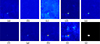 |
Fig. 11 The detection results of different methods on the dataset (Jungle-I). (a) RX; (b) 2S-GLRT; (c) CRD; (d) RGAE; (e) Auto-AD; (f) CTA; (g) GT-HAD; (h) TAEF; (i) Proposed method; (j) Ground-truth maps. |
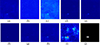 |
Fig. 12 The detection results of different methods on the dataset (Jungle-II). (a)RX; (b) 2S-GLRT; (c) CRD; (d) RGAE; (e) Auto-AD; (f) CTA; (g) GT-HAD; (h) TAEF; (i) Proposed method; (j) Ground-truth maps. |
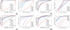 |
Fig. 13 ROC curve(left) and log scale ROC curve (right) of detection results. (a) Holly. (b) Cement Street. (c) Jungle-I. (d) Jungle-II. |
AUC of different methods on different data.
5 Conclusion
This paper proposes a novel dual-window transformer framework featuring a pyramid structure and constrained self-attention for hyperspectral image anomaly detection. The core innovation lies in its ability to extract deep spectral differences between central pixels and their surrounding background through the dual-window transformer. A specifically designed constrained self-attention mechanism enhances this process. Furthermore, the pyramid structure integrates global contextual information from its upper layers into the CASTM, achieving an effective fusion of local and global information. This hierarchical design also significantly mitigates the impact of dual-window size selection on the model’s performance, thereby improving the framework’s overall robustness. Comprehensive parameter analyses across four collected datasets validate the robustness of the proposed method. Comparative experiments demonstrate that our method is particularly well-suited for hyperspectral imagery characterized by complex scenes and significant spectral uncertainty, achieving a higher detection rate. These results confirm the method’s rationality and superiority. Essentially, our approach represents a hybrid of dual-window training-based and reconstruction-based paradigms, successfully integrating both global and local anomalous information. This integration offers a novel and effective strategy for enhancing HAD performance. The proposed method shows great promise for practical applications, such as large-area reconnaissance and preliminary screening prior to precise target identification. Future work will focus on two primary objectives: reducing the false alarm rate and further improving the computational efficiency of the framework.
Funding
This research did not receive any specific funding.
Conflicts of interest
The authors declare that they have no competing interests to report.
Data availability statement
Some hyperspectral images used in this paper are public data sets commonly used in the field, which can be obtained from the Internet according to the description of the data set in this paper. The remaining dataset was taken by the author themselves and can be obtained or inquired about through email.
Author contribution statement
All authors have reviewed, discussed, and agreed to their personal contributions. The specific situation is as follows: Conceptualization, Bing Zhou; Methodology, Algorithms, Analysis and Writing, Lei Deng; Data visualization and Review, Zhaorui Li.
References
- Su H, Wu Z, Zhang H, Du Q, Hyperspectral anomaly detection: a survey, IEEE Geosci. Remote Sens. Mag. 10, 64–90 (2022). https://doi.org/10.1109/MGRS.2021.3105440. [Google Scholar]
- Xu Y, Zhang L, Du B, Zhang L, Hyperspectral anomaly detection based on machine learning: an overview, IEEE J. Sel. Top. Appl. Earth Obs. Remote. Sens. 15, 3351–3364 (2022). https://doi.org/10.1109/JSTARS.2022.3167830. [Google Scholar]
- Xie W, Fan S, Qu J, Wu X, Lu Y, Du Q, Spectral distribution-aware estimation network for hyperspectral anomaly detection, IEEE Geosci. Remote Sens. Mag. 60, 5512312 (2022). https://doi.org/10.1109/TGRS.2021.3089711. [Google Scholar]
- Zhao C, Li C, Feng S, Li W, Spectral-spatial anomaly detection via collaborative representation constraint stacked autoencoders for hyperspectral images, IEEE Geosci. Remote Sens. Lett. 19, 5503105 (2022). https://doi.org/10.1109/LGRS.2021.3050308. [Google Scholar]
- Zhao R, Yang Z, Meng X, Shao F, A novel fully convolutional auto-encoder based on dual clustering and latent feature adversarial consistency for hyperspectral anomaly detection, Remote Sens. 16, 717 (2024). https://doi.org/10.3390/rs16040717. [Google Scholar]
- Hu X, Xie C, Fan Z, Duan Q, Zhang D, Jiang L, Wei X, Hong D, Li G, Zeng X, Hyperspectral anomaly detection using deep learning: a review, Remote Sens. 14, 1973 (2022). https://doi.org/10.3390/rs14091973. [Google Scholar]
- Zhang JJ, Xiang P, Shi J, Teng X, Zhao D, Zhou HX, Li H, Song JL, A light CNN based on residual learning and background estimation for hyperspectral anomaly detection, Int. J. Appl. Earth Obs. Geoinf. 132, 104069 (2024). https://doi.org/10.1016/j.jag.2024.104069. [Google Scholar]
- Cheng X, Deep feature aggregation network for hyperspectral anomaly detection, IEEE Trans. Instrum. Meas. 73, 5033016 (2024). https://doi.org/10.1109/TIM.2024.3403211. [Google Scholar]
- Reed IS, Yu X, Adaptive multiple-band CFAR detection of an optical pattern with unknown spectral distribution, IEEE Trans. Acoust. Speech Signal Process. 38, 1760–1770 (1990). https://doi.org/10.1109/29.60107. [Google Scholar]
- Kwon H, Der SZ, Nasrabadi NM, Adaptive anomaly detection using subspace separation for hyperspectral imagery, Opt. Eng. 42, 3342–3351 (2003). https://doi.org/10.1117/1.1614265. [Google Scholar]
- Guo Q, Zhang B, Ran Q, Gao L, Li J, Plaza A, Weighted-RXD and linear filter-based RXD: improving background statistics estimation for anomaly detection in hyperspectral imagery, IEEE J. Sel. Top. Appl. Earth Obs. Remote Sens. 7, 2351–2366 (2014). https://doi.org/10.1109/JSTARS.2014.2302446. [Google Scholar]
- Liu J, Hou Z, Li W, Tao R, Orlando D, Li H, Multipixel anomaly detection with unknown patterns for hyperspectral imagery, IEEE Trans. Neur. Netw. Learn. Syst. 33, 5557–5567 (2022). https://doi.org/10.1109/TNNLS.2021.3071026. [Google Scholar]
- Ling Q, Guo Y, Lin Z, An W, A constrained sparse representation model for hyperspectral anomaly detection, IEEE Geosci. Remote Sens. Mag. 57, 2358–2371 (2019). https://doi.org/10.1109/TGRS.2018.2872900. [Google Scholar]
- Li W, Du Q, Collaborative representation for hyperspectral anomaly detection, IEEE Geosci. Remote Sens. Mag. 53, 1463–1474 (2015). https://doi.org/10.1109/TGRS.2014.2343955. [Google Scholar]
- Sun W, Liu C, Li J, Lai YM, Li W, Low-rank and sparse matrix decomposition-based anomaly detection for hyperspectral imagery, J. Appl. Remote Sens. 8, 083641 (2014). https://doi.org/10.1117/1.jrs.8.083641. [Google Scholar]
- Kang X, Zhang X, Li S, Li K, Li J, Benediktsson JA, Hyperspectral anomaly detection with attribute and edge-preserving filters, IEEE Geosci. Remote Sens. Mag. 55, 5600–5611 (2017). https://doi.org/10.1109/TGRS.2017.2710145. [Google Scholar]
- Li W, Wu G, Du Q, Transferred deep learning for anomaly detection in hyperspectral imagery, IEEE Geosci. Remote Sens. Lett. 14, 597–601 (2017). https://doi.org/10.1109/LGRS.2017.2657818. [Google Scholar]
- Batı E, Çalışkan A, Koz A, Alatan AA, Hyperspectral anomaly detection method based on auto-encoder, Image Signal Process. Remote Sens. 9643, 1–7 (2015). https://doi.org/10.1117/12.2195180. [Google Scholar]
- Wang S, Wang X, Zhang L, Zhong Y, Auto-AD: autonomous hyperspectral anomaly detection network based on fully convolutional autoencoder, IEEE Geosci. Remote Sens. Mag. 60, 5503314 (2022). https://doi.org/10.1109/TGRS.2021.3057721. [Google Scholar]
- Fan G, Ma Y, Mei X, Fan F, Huang J, Ma J, Hyperspectral anomaly detection with robust graph autoencoders, IEEE Geosci. Remote Sens. Mag. 60, 5511314 (2022). https://doi.org/10.1109/TGRS.2021.3097097. [Google Scholar]
- Liu H, Su X, Shen X, Zhou C, Chen X, Zhou X, BiGSeT: binary mask-guided separation training for dnn-based hyperspectral anomaly detection (2023). https://doi.org/10.48550/arXiv.2307.07428. [Google Scholar]
- Ma D, Chen M, Yang Y, Li B, Li M, Gao Y, Coarse-to-fine multiview anomaly coupling network for hyperspectral anomaly detection, IEEE Geosci. Remote Sens. Mag. 62, 5507715 (2024). https://doi.org/10.1109/TGRS.2024.3362055. [Google Scholar]
- Wu ZY, Wang B, Background reconstruction via 3D-transformer network for hyperspectral anomaly detection, Remote Sens. 15, 4592 (2023). https://doi.org/10.3390/rs15184592. [Google Scholar]
- Xiao S, Zhang T, Xu Z, Qu J, Hou S, Dong W, Anomaly detection of hyperspectral images based on transformer with spatial-spectral dual-window mask, IEEE J. Sel. Top. Appl. Earth Obs. Remote Sens. 16, 1414–1426 (2023). https://doi.org/10.1109/JSTARS.2022.3232762. [Google Scholar]
- Lian J, Wang L, Sun H, Huang H, GT-HAD: gated transformer for hyperspectral anomaly detection, IEEE Trans. Neural Netw. Learn. Syst. 36, 3631–3645 (2025). https://doi.org/10.1109/TNNLS.2024.3355166. [Google Scholar]
- Wang Z, Ma D, Yue G, Li B, Cong R, Wu Z, Self-supervised hyperspectral anomaly detection based on finite spatialwise attention, IEEE Geosci. Remote Sens. Mag. 62, 5502918 (2024). https://doi.org/10.1109/TGRS.2023.3347270. [Google Scholar]
- Zhang J, Xiang P, Teng X, Zhao D, Li H, Song J, Zhou H, Tan W, Enhancing hyperspectral anomaly detection with a novel differential network approach for precision and robust background suppression, Remote Sens. 16, 434 (2024). https://doi.org/10.3390/rs16030434. [Google Scholar]
- Li K, An W, Wang Y, Zhang T, Qin Y, Gao T, Explicit background endmember learning for hyperspectral anomaly detection, IEEE Trans. Instrum. Meas. 73, 5028817 (2024). https://doi.org/10.1109/TIM.2024.3446609. [Google Scholar]
- He Z, He D, Xiao M, Lou A, Lai G, Convolutional transformer-inspired autoencoder for hyperspectral anomaly detection, IEEE Geosci. Remote Sens. Lett. 20, 5508905 (2023). https://doi.org/10.1109/LGRS.2023.3312589. [Google Scholar]
- Liu S, Peng L, Chang X, Wang Z, Wen G, Zhu C, Adaptive dual-domain learning for hyperspectral anomaly detection with state-space models, IEEE Geosci. Remote Sens. Mag. 63, 5503719 (2025). https://doi.org/10.1109/TGRS.2025.3530397. [Google Scholar]
- Sun X, Zhang Y, Dong Y, Du B, Contrastive self-supervised learning-based background reconstruction for hyperspectral anomaly detection, IEEE Geosci. Remote Sens. Mag. 63, 5504312 (2025). https://doi.org/10.1109/TGRS.2025.3534185. [Google Scholar]
- Guo Q, Cen Y, Zhang L, Zhang Y, Huang Y, Hyperspectral anomaly detection based on spatial–spectral cross-guided mask autoencoder, IEEE J. Sel. Top. Appl. Earth Obs. Remote Sens. 17, 9876–9889 (2024). https://doi.org/10.1109/JSTARS.2024.3393995. [Google Scholar]
- Liu S, Guo H, Gao S, Zhang W, The spectrum difference enhanced network for hyperspectral anomaly detection, Remote Sens. 16, 4518 (2024). https://doi.org/10.3390/rs16234518. [Google Scholar]
- Wu Z, Wang B, Transformer-based autoencoder framework for nonlinear hyperspectral anomaly detection, IEEE Geosci. Remote Sens. Mag. 62, 5508015 (2024). https://doi.org/10.1109/TGRS.2024.3361469. [Google Scholar]
- Young SS, Lin CH, Leng ZC, Unsupervised abundance matrix reconstruction transformer-guided fractional attention mechanism for hyperspectral anomaly detection, IEEE Trans. Neural Netw. Learn. Syst. 36, 9150–9164 (2025). https://doi.org/10.1109/TNNLS.2024.3437731. [Google Scholar]
- Xu YT, Zhao K, Zhang LG, Zhu MY, Zeng D, Hyperspectral anomaly detection with vision transformer and adversarial refinement, Inter. J. Remote Sens. 44, 4034–4057 (2023). https://doi.org/10.1080/01431161.2023.2229495. [Google Scholar]
- Li Z, Wang Y, Xiao C, Ling Q, Lin Z, An W, You only train once: learning a general anomaly enhancement network with random masks for hyperspectral anomaly detection, IEEE Geosci. Remote Sens. Mag. 61, 5506718 (2023). https://doi.org/10.1109/TGRS.2023.3258067. [Google Scholar]
- Wang J, Ouyang T, Duan Y, Cui L, SAOCNN: self-attention and one-class neural networks for hyperspectral anomaly detection, Remote Sens. 14, 5555 (2022). https://doi.org/10.3390/rs14215555. [Google Scholar]
- Wang X, Wang L, Wang Q, Local spatial–spectral information-integrated semisupervised two-stream network for hyperspectral anomaly detection, IEEE Geosci. Remote Sens. Mag. 60, 5535515 (2022). https://doi.org/10.1109/TGRS.2022.3196409. [Google Scholar]
- Duan Y, Ouyang T, Wang J, CRNN: collaborative representation neural networks for hyperspectral anomaly detection, Remote Sens. 15, 3357 (2023). https://doi.org/10.3390/rs15133357. [Google Scholar]
- Wang X, Hyperspectral anomaly detection using dual-branch network based on frequency domain learning, IEEE J. Sel. Top. Appl. Earth Obs. Remote Sens. 18, 15789–15803 (2025). https://doi.org/10.1109/JSTARS.2025.3580575. [Google Scholar]
- Wang J, Sun J, Xia Y, Zhang Y, Dynamic negative sampling autoencoder for hyperspectral anomaly detection, IEEE J. Sel. Top. Appl. Earth Obs. Remote Sens. 15, 9829–9841 (2022). https://doi.org/10.1109/JSTARS.2022.3220514. [Google Scholar]
- Vaswani A, Shazeer N, Parmar N, Uszkoreit J, Jones L, Gomez AN, Kaiser L, Polosukhin I, Attention is all you need (2023). https://doi.org/10.48550/arXiv.1706.03762. [Google Scholar]
- Dosovitskiy A, Beyer L, Kolesnikov A, Weissenborn D, Zhai XH, Unterthiner T, Dehghani M, Minderer M, Heigold G, Gelly S, Uszkoreit J, Houlsby N, An image is worth 16 × 16 words: transformers for image recognition at scale (2021). https://doi.org/10.48550/arXiv.2010.11929. [Google Scholar]
- Hu X, Li ZX, Karimi HR, Zhang DW, Dictionary trained attention constrained low rank and sparse autoencoder for hyperspectral anomaly detection, Neural Netw. 181, 106797 (2023). https://doi.org/10.1016/j.neunet.2024.106797. [Google Scholar]
All Tables
All Figures
|
Fig. 1 The calculation process of multi-head attention. |
| In the text | |
|
Fig. 2 Diagram of stacked autoencoder (SAE). |
| In the text | |
|
Fig. 3 Framework of the proposed method. |
| In the text | |
|
Fig. 4 Diagram of intrinsic constraints. |
| In the text | |
|
Fig. 5 Pseudocolor images (left) and the corresponding ground-truth maps (right) of five real hyperspectral datasets. (a) Meadow; (b) Holly; (c) Cement Street; (d) Jungle-I; (e) Jungle-II. |
| In the text | |
|
Fig. 6 AUC under different dual-windows when heads = 1. |
| In the text | |
|
Fig. 7 AUC under different numbers of heads when depth = 5. |
| In the text | |
|
Fig. 8 AUC under different depths when heads = 6. |
| In the text | |
|
Fig. 9 The detection results of different methods on the dataset (Holly). (a) RX; (b) 2S-GLRT; (c) CRD; (d) RGAE; (e) Auto-AD; (f) CTA; (g) GT-HAD; (h) TAEF; (i) Proposed method; (j) Ground-truth maps. |
| In the text | |
|
Fig. 10 The detection results of different methods on the dataset (Cement Street). (a) RX; (b) 2S-GLRT; (c) CRD; (d) RGAE; (e) Auto-AD; (f) CTA; (g) GT-HAD; (h) TAEF; (i) Proposed method; (j) Ground-truth maps. |
| In the text | |
|
Fig. 11 The detection results of different methods on the dataset (Jungle-I). (a) RX; (b) 2S-GLRT; (c) CRD; (d) RGAE; (e) Auto-AD; (f) CTA; (g) GT-HAD; (h) TAEF; (i) Proposed method; (j) Ground-truth maps. |
| In the text | |
|
Fig. 12 The detection results of different methods on the dataset (Jungle-II). (a)RX; (b) 2S-GLRT; (c) CRD; (d) RGAE; (e) Auto-AD; (f) CTA; (g) GT-HAD; (h) TAEF; (i) Proposed method; (j) Ground-truth maps. |
| In the text | |
|
Fig. 13 ROC curve(left) and log scale ROC curve (right) of detection results. (a) Holly. (b) Cement Street. (c) Jungle-I. (d) Jungle-II. |
| In the text | |
Current usage metrics show cumulative count of Article Views (full-text article views including HTML views, PDF and ePub downloads, according to the available data) and Abstracts Views on Vision4Press platform.
Data correspond to usage on the plateform after 2015. The current usage metrics is available 48-96 hours after online publication and is updated daily on week days.
Initial download of the metrics may take a while.