| Issue |
J. Eur. Opt. Society-Rapid Publ.
Volume 19, Number 2, 2023
|
|
|---|---|---|
| Article Number | 45 | |
| Number of page(s) | 12 | |
| DOI | https://doi.org/10.1051/jeos/2023045 | |
| Published online | 22 December 2023 | |
Research Article
Spectral reflectance fitting based on land-based hyperspectral imaging and semi-empirical kernel-driven model for typical camouflage materials
1
Department of Electronic and Optical Engineering, Shijiazhuang Campus, Army University of Engineering, Shijiazhuang 050000, China
2
Department of Missile Engineering, Shijiazhuang Campus, Army University of Engineering, Shijiazhuang 050000, China
* Corresponding author: This email address is being protected from spambots. You need JavaScript enabled to view it.
Received:
19
October
2023
Accepted:
7
December
2023
Abstract
The reflectance of an object is a physical quantity that is related to a variety of factors such as wavelength, direction of light source, direction of detection, and weather conditions. If complete spectral information about the target is to be obtained, this can only be done by measuring the spectral reflectance in all angular directions. Obviously, this method of acquiring spectral data has the disadvantages of complex operation, low efficiency and poor timeliness in military applications. The Semi-Empirical kernel-driven model captures the main factors affecting the bidirectional reflective properties of an object and uses physically meaningful kernel parameters to characterise the reflective properties of an object. By measuring these kernel parameters and combining them with a small number of measurements, it is possible to extrapolate and fit the spectral reflectance of the target in all directions, improving the efficiency of information acquisition and processing. Semi-empirical kernel-driven models were initially used to study the composition and structure of vegetation and its spectral reflectance properties with some results. However, whether the semi-empirical kernel-driven model can be effectively used to study the spectral reflectance properties of military materials has not been verified. This paper first introduces three commonly used semi-empirical kernel-driven models, namely RossThick-LiSparseR (RTLSR), RossThick-LiTransitN (RTLT) and RossThick-Roujean (RTR). Then, the spectral reflectance of four typical military materials was measured using an imaging spectrometer, and the fitting effects of different models were evaluated. Experiments show that the three semi-empirical kernel-driven models have good data fitting ability for different types of military materials. Overall, RTLSR model has the best data fitting ability and the best stability of inversion results.
Key words: Hyperspectral imaging / Spectral reflectance / Military materials / Semi-empirical kernel-driven model
© The Author(s), published by EDP Sciences, 2023
 This is an Open Access article distributed under the terms of the Creative Commons Attribution License (https://creativecommons.org/licenses/by/4.0), which permits unrestricted use, distribution, and reproduction in any medium, provided the original work is properly cited.
1 Introduction
Spectral information of ground objects can break through the limitation of two-dimensional space and explain the characteristics of objects from a spectral perspective. With the rapid development of hyperspectral imaging technology, specific spectral information greatly improves the efficiency of target classification [1, 2] and detection [3, 4]. Imaging spectroscopy was first applied in the field of remote sensing, with relatively stable detection methods and conditions. However, the acquisition of spectral reflectance information of ground objects requires complex pre-processing processes, such as radiometric calibration and atmospheric correction. In addition, the problem of “the same spectrum but different objects or the same object but different spectra” is significant in the traditional remote sensing hyperspectral detection [5]. The reflections of most objects in nature are anisotropic. In near-ground quantitative spectral measurements, the interaction between ground objects and electromagnetic waves has a more obvious effect. Therefore, the bidirectional reflection distribution function (BRDF) model is often established to describe the spectral reflection characteristics of ground objects in all directions [6]. In the 1970s, Nicodemus proposed the precise definition of the BRDF, and the research of BRDF model has also made great progress. Various models with different complexity, characteristics and advantages have emerged. Researchers at home and abroad have combined mathematical physics methods with applications to establish a variety of BRDF models. These models can be divided into statistical model, physical model and semi-empirical model according to different construction methods. The semi-empirical kernel-driven model is a typical BRDF model, which is widely used in industry [7], agriculture [8], environmental monitoring [9, 10], and other fields due to its simplicity and strong fitting ability.
In the military field, the development of hyperspectral technology has effectively improved the accuracy and reliability of reconnaissance and has been widely used in camouflaged targets [11], mines [12], and near-sea detection [13]. Hyperspectral reconnaissance technology achieves the detection of weak changes in spectral features between true and false targets, targets and camouflage, and coverings and the normal surrounding environment through the quantitative analysis of spectral features. It is capable of accomplishing target localisation and has become a new and important reconnaissance tool [14]. However, it is critical to establish a spectral database of various military materials in order to fulfill hyperspectral reconnaissance missions. How to obtain all-round accurate spectral reflectance information of targets conveniently and quickly has become an urgent problem. Currently, despite the rapid development of semi-empirical kernel-driven models, there have been no studies demonstrating their ability to accurately fit and invert multi-angle reflectance information for military materials.
This paper first introduces the principle of BRDF model and the typical semi-empirical kernel-driven model. Then the method and process of spectral reflectance measurement of ground objects are described. A fitted similarity assessment method that integrates spectral angular distance and correlation is presented. Spectral reflectance data of typical military materials were obtained by field experiments. Three different semi-empirical kernel-driven models were used for fitting and the models were analysed for their goodness of fit to the measured data. This study not only shows that the semi-empirical kernel-driven model has a wide range of applications but also provides ideas for establishing and expanding a spectral database for military materials.
2 Basic theory
2.1 BRDF model
BRDF extracts the geometric radiation relationship among the light source, target and detector in the spectral detection of ground objects. Therefore, BRDF model is often used to study the directional reflection characteristics of ground objects. Its formula is shown in formula (1): (1)where θ
i
and φ
i
represent the zenith angle and azimuth of the incident sunlight. θ
r
and φ
r
represent the zenith angle and azimuth of the reflected light. λ represents the wavelength of the incident light. dE
i
represents the incident irradiance of the light source on the panel near the incident point and dL
r
is the irradiance in the corresponding reflection direction. The schematic diagram of BRDF is shown in Figure 1.
(1)where θ
i
and φ
i
represent the zenith angle and azimuth of the incident sunlight. θ
r
and φ
r
represent the zenith angle and azimuth of the reflected light. λ represents the wavelength of the incident light. dE
i
represents the incident irradiance of the light source on the panel near the incident point and dL
r
is the irradiance in the corresponding reflection direction. The schematic diagram of BRDF is shown in Figure 1.
 |
Figure 1 BRDF schematic diagram. |
However, the conditions for measuring the BRDF of a target are very harsh. In order to meet the measurement requirements, a bidirectional reflectance factor (BRF) is often used to replace the measurement of BRDF. BRF describes the ratio of the reflected radiance value in the direction of the ground object to the radiance value of the ideal diffuse reflector which is expressed in R. Its mathematical expression is: (2)where dL
r
is the reflected radiance value of the ground object in θ
r
and φ
r
directions. dL
p
is the reflected radiance value of the ideal diffuse reflector in this direction under the same conditions. φ = |φ
i
– φ
r
| is the relative azimuth angle between the light source and the detector.
(2)where dL
r
is the reflected radiance value of the ground object in θ
r
and φ
r
directions. dL
p
is the reflected radiance value of the ideal diffuse reflector in this direction under the same conditions. φ = |φ
i
– φ
r
| is the relative azimuth angle between the light source and the detector.
Semi-empirical models capture the main factors affecting BRDF and are widely used in batch processing algorithms. Its representative kernel-driven model is fitted by the linear combination of kernel with certain physical significance. The parameters of the model are the combination of weights for the isotropic uniform scattering kernel, the volume scattering kernel and the geometrical optical scattering kernel, reflecting the three main types of surface scattering. The specific formula is as follows: (3)
(3)
The model decomposes the dichroic reflection into a linear combination of three components, where R s represents the dichroic reflectance under direct light source. Kvol and Kgeo are volume scattering kernel and geometric optical kernel, respectively. The volume scattering kernel is derived from the classical radiation transfer theory, mainly including the RossThick kernel and RossThin kernel. Shadow and mutual shadowing effects are considered in geometrical optical kernel, mainly including the LiSparse kernel, LiDense kernel, LiSparseR kernel, LiTransitN kernel and Roujean kernel. fiso(λ), fvol(λ) and fgeo(λ) are only related to the wavelength, and represent the proportions of uniform scattering, volume scattering and geometrical optical scattering, respectively.
The volume scattering kernel and the geometrical optical kernel are only related to the directional conditions of the light source and the detector, and can be calculated by the detection angle, azimuth angle and solar altitude angle. When calculating the reflectance, the values of the two cores can be calculated first since the integration of the two cores is independent of the constant coefficient. The values of the three constant coefficients can be obtained by substituting the existing reflectance data and the values of the two cores into the linear fitting, and then the reflectance of the ground object under any direction can be extrapolated.
The RTLSR model, RTLT model and RTR model are used in this study. The difference between these three typical kernel-driven models is mainly that the geometric optical scattering kernel are selected differently, and the selected volume scattering kernel are RossThick kernel. These three models are applicable to different application scenarios, and the detailed theoretical derivation process of the model is open, so I will not repeat it.
The expression for RossThick kernel is as follows: (4)
(4)
Among them, δ is the phase angle that satisfies formula (5): (5)
(5)
The geometric optical scattering kernel of RTLSR is LiSparseR. The expression for LiSparseR kernel is as follows: (6)
(6)
 (7)
(7)
 (8)
(8)
 (9)
(9)
The geometric optical scattering kernel of RTLT is LiTransitN. The expression for LiTransitN kernel is as follows: (10)
(10)
 (11)
(11)
 (12)
(12)
 (13)
(13)
The geometric optical scattering kernel of RTR is Roujean. The expression for Roujean kernel is as follows:![Mathematical equation: $$ {K}_{\mathrm{Roujean}}\left({\theta }_i,{\theta }_r,\phi \right)=\frac{1}{2\pi }\left[\left(\mathrm{\pi }-\phi \right)\mathrm{cos}\phi +\mathrm{sin}\phi \right]\mathrm{tan}{\theta }_i-\frac{1}{\pi }\left(\mathrm{tan}{\theta }_i+\mathrm{tan}{\theta }_r+\sqrt{{\mathrm{tan}}^2{\theta }_i-{\mathrm{tan}}^2{\theta }_r-2\mathrm{tan}{\theta }_i\mathrm{tan}{\theta }_r\mathrm{cos}\phi }\right). $$](/articles/jeos/full_html/2023/02/jeos20230055/jeos20230055-eq14.gif) (14)
(14)
2.2 Acquisition of object ground spectral reflectance
Reflectivity is defined as the ratio of the energy value reflected by the object surface to the incident energy value reaching the object surface. Spectral reflectance is the reflectance of an object measured at a specific wavelength. Continuous measurement constitutes the reflectance spectrum of an object. When measuring the spectral reflectance of objects in the near ground, there are two main transmission processes to consider. One is the process by which direct sunlight hits a ground object and is reflected by the object to the detector, and the other is the process by which diffuse light from the surrounding area hits the object and is reflected back to the detector. The incident light of sunlight on the ground can be regarded as directional incident parallel light. The light reflected by the surrounding features and reaching the features is approximately hemispherical. Therefore, the BRF of the object can be expressed by the weighted sum of the two.As shown in formula (15): (15)
(15)
θ i represents the zenith angle of the sun. φ i represents the azimuth of the sun. θ r represents the zenith angle of the observation instrument. φ r represents the azimuth angle of the observation instrument. R D (θ r, φ r ) represents the reflectance of the diffuse incident hemisphere in a certain direction. R s (θ i, φ i; θ r, φ r ) represents the bidirectional reflectance under direct sunlight. R(θ i, φ i; θ r, φ r ) represents the total reflectance measured under land-based conditions. It is difficult to directly measure the proportion of directional incident light action K1 and hemispherical incident light action K2, respectively. Therefore, the value K2 represented by the ratio of the brightness value of the standard white board under shadow and sunlight is often used to calculate the K1 value according to K1 = 1 −K2. The measurement process is shown schematically in Figure 2.
 |
Figure 2 Schematic diagram of measurement process. (a) Unobstructed condition; (b) Blocked condition. |
According to formula (15):![Mathematical equation: $$ {R}_s\left({\theta }_i,{\phi }_i;{\theta }_r,{\phi }_r\right)=\left[R\left({\theta }_i,{\phi }_i;{\theta }_r,{\phi }_r\right)-{K}_2{R}_{\mathrm{D}}\left({\theta }_r,{\phi }_r\right)\right]\div {K}_1. $$](/articles/jeos/full_html/2023/02/jeos20230055/jeos20230055-eq16.gif) (16)
(16)
Therefore, the value of R s can be calculated by measuring other physical quantities, substituted into formula (3).The corresponding model parameters can be obtained by using the least square method. Fitted reflectance curves can be obtained by applying known model parameters to the reflectance inversion. Comparison of the fitted reflectivity curves with the experimental data makes it possible to evaluate the fit obtained with different models.
3 Evaluation index of spectral curve fitting effect
3.1 Spectral correlation coefficient (SCC)
The correlation coefficient can reflect the correlation between two variables and their correlation direction. It is within the interval [−1, 1]. When the correlation coefficient is −1, it indicates that the two variables to be observed change in exactly opposite directions and magnitudes. When the correlation coefficient is 1, it indicates that the change direction and amplitude of the two variables to be observed are identical. When the correlation coefficient is 0, it means that the two are not related. The correlation coefficient of two variables
X
and
Y
is often expressed by r. The greater the correlation r, the stronger the correlation. The specific expression is formula (17). (17)
(17)
It should be pointed out that the correlation coefficient has an obvious disadvantage. The correlation coefficient can only reflect the trend of the two variables, that is, it cannot accurately indicate the degree of deviation between the two variables.
3.2 Spectral angle cosine (SAC)
Spectral angle cosine uses the shape measurement between spectral curves. The cosine value of the spectral angle reflects the cosine value of the generalized included angle of the two vectors which reflects the similarity of the two curves to a certain extent. The value range of the spectral angle cosine value is [0, 1]. The larger the value, the more similar the two vectors are. The specific expression of the SAC value of the two variables
X
and
Y
is formula (18). (18)where θ is the generalized included angle of two variables. However, the similarity evaluation index based on the generalized angle of spectrum is difficult to complete the similarity evaluation of linear correlation vectors.
3.3 Measurement method considering SCC and SAC comprehensively
A single spectral similarity metric is often flawed in that it utilises only one aspect of the spectral profile. It has been proved that the combination of two or more similarity measures can effectively evaluate the accuracy of fitting two spectral curves. Therefore, a spectral angle cosine correlation coefficient measure is proposed in this paper. The arithmetic mean is used to combine the two similarity measures and the result is expressed in CSS: (19)
(19)
Obviously, the value range of CSS measure is [0, 1]. The larger the value of CSS, the more similar the spectral curves are and the better the fitting effect is.
3.4 Standard deviation
Standard deviation (StDev) is a common concept in statistics. Standard deviation is defined as the arithmetic square root of variance. The standard deviation is usually represented by S, as shown in formula (20): (20)
(20)
The smaller the StDev, the stronger the stability of the model inversion result and the closer the inversion result is to the measured data.
4 Experiments
4.1 Experimental data
The detection instrument selected in the experiment is a field imaging spectrometer based on acousto-optical tunable filer (AOTF), which can simultaneously obtain spatial information and continuous spectral information. The working band of the spectrometer is the visible light band, and the spectral resolution is set at 4nm. In the wavelength range of 449–801 nm, 89 greyscale images of different bands can be obtained. Each image records the radiation intensity of the ground objects in different bands. The experimental time is April 27, 2022. The experimental site is a certain place in Shijiazhuang City, Hebei Province, China. The longitude and latitude are 38°27′ N, 114°30′ E. The altitude is 78 m above sea level. Four groups of spectral reflectance measurement experiments of ground objects were carried out at four different times. The specific conditions, solar altitude, zenith angle, relative azimuth and other data are shown in Table 1. A total of four sets of data were obtained under different conditions. Four typical military materials were selected for the test, namely, jungle green camouflage uniform, desert grey camouflage uniform, desert grey camouflage steel plate and jungle green camouflage steel plate. These four types of objects are marked as A, B, C and D respectively. The schematic diagram of the placement of experimental objects is shown in Figuer 3. Figure 4 refers to a hyperspectral single band scene obtained by using an imaging spectrometer.
 |
Figure 3 Placement of experimental objects. |
 |
Figure 4 Single band grayscale image of experimental scene. |
Experimental measurement conditions.
The white plate used in the experiment is a metered and calibrated polytetrafluoroethylene plate (PTFE). The reflection characteristics of the PTEE material in all directions are relatively uniform, which can be roughly seen as a Lambertian body. In order to obtain the directional reflectance factor under direct sunlight, first measure the total directional reflectance factor in the field, and then measure the directional reflectance factor in a specific direction caused by hemispherical incidence in the case of obstructions. Substitute all parameters into formula (16) to get R s .
4.2 Data analysis
In order to study the influence of solar altitude angle change on the spectral curve of typical military materials, the R s of four military materials A, B, C and D under direct light at different times are compared, as shown in Figure 5.
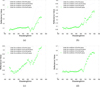 |
Figure 5 Bidirectional reflectance factors of four military materials (A, B, C, D) under different conditions of direct light. (a) Bidirectional reflectance factor of object A under different conditions of direct light; (b) Bidirectional reflectance factor of object B under different conditions of direct light; (c) Bidirectional reflectance factor of object C under different conditions of direct light; (d) Bidirectional reflectance factor of object D under different conditions of direct light. |
It can be seen from the experimental results that the basic laws of the spectral curves of the four research objects with the change of angular conditions are the same. Although there are some differences in the spectral reflectance curves of the same feature under different direction conditions, they are almost the same in terms of numerical values and change trends. From the perspective of research objects, the spectral reflectance of objects A and B fluctuates relatively large with the change of direction conditions, while the spectral reflectance of objects C and D fluctuates relatively small with the change of direction conditions. This phenomenon may be caused by the rough surfaces of objects A and B, which have significant bi-directional reflective properties, while the surfaces of objects C and D are relatively flat.
It can be seen from formula (3) that the semi-empirical kernel-driven model requires at least three sets of a priori reflectivity data and directional angle conditions to complete the measurement of model parameters. In order to make the experimental results more convincing, this paper uses the four groups of experimental data obtained in the experiment for cross validation. The first, third and fourth groups of experimental data are used as a priori data to fit the target spectral reflectance in the second group of experiments. The first, second and fourth sets of experimental data are used as a priori data to fit the target spectral reflectance in the third set of experiments. The first, second and third sets of experimental data are used as a priori data to fit the target spectral reflectance in the fourth set of experiments. The RTLSR model, RTLT model and RTR model are used to fit the spectral reflectance of four typical military materials: A, B, C and D. The experimental results are shown in Figures 6–8.
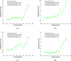 |
Figure 6 Group 1, 3 and 4 data to verify group 2 data. Using RTLSR, RTLT and RTR model, the spectral reflectance of four typical military materials A, B, C and D are fitted respectively. (a) Fitting results of spectral reflectance of object A with different models; (b) Fitting results of spectral reflectance of object B with different models; (c) Fitting results of spectral reflectance of object C with different models; (d) Fitting results of spectral reflectance of object D with different models. |
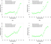 |
Figure 7 Group 1, 2 and 4 data to verify group 3 data. Using RTLSR, RTLT and RTR model, the spectral reflectance of four typical military materials A, B, C and D are fitted respectively. (a) Fitting results of spectral reflectance of object A with different models; (b) Fitting results of spectral reflectance of object B with different models; (c) Fitting results of spectral reflectance of object C with different models; (d) Fitting results of spectral reflectance of object D with different models. |
 |
Figure 8 Group 1, 2 and 3 data to verify group 4 data. Using RTLSR, RTLT and RTR model, the spectral reflectance of four typical military materials A, B, C and D are fitted respectively. (a) Fitting results of spectral reflectance of object A with different models; (b) Fitting results of spectral reflectance of object B with different models; (c) Fitting results of spectral reflectance of object C with different models; (d) Fitting results of spectral reflectance of object D with different models. |
First, through qualitative analysis of the fitting data, it is obvious that the three semi-empirical kernel-driven models used in this paper have good effects in the inversion of surface reflectance. From the perspective of these four kinds of surface features, the fitting effect of various models on D object is better. However, in order to further compare the fitting ability of RTLSR model, RTLT model and RTR model to the spectral reflectance of four typical military materials, A, B, C and D, it is necessary to quantitatively analyze the experimental results. SCC, SAC, CSS and StDev were used for evaluation. Among them, the value range of SCC, SAC and CSS is [0, 1]. The closer to 1, the better the fitting effect. StDev can reflect the deviation of the model fitting results. The smaller the value, the better the stability of the model in the fitting process. The experimental results are shown in Table 2.
Evaluation of spectral reflectance fitting results of different models for A, B, C and D.
Based on the above experimental evaluation results, Table 3 lists the minimum value of CSS (indicating that in the same feature and different models, the CSS value of this model is the minimum), the second minimum value of CSS (indicating that in the same feature and different models, the CSS value of this model is between the maximum and minimum), and the maximum value of CSS (indicating that in the same feature and different models, the CSS value of this model is the maximum). Table 4 shows the statistics of the values of StDev for the three models. The statistical methods are the same as those of CSS values.
CSS numerical statistics of different models.
StDev numerical statistics of different models.
At the same time, in order to study the fitting effect of different types of ground objects, Table 5 lists the minimum value of CSS (indicating that in different objects and the same model, the CSS value of this type of object is the minimum), the second small value of CSS (indicating that in different objects and the same model, the CSS value of this type of object is only greater than the minimum), the second large value of CSS (indicating that in different objects and the same model, the CSS value of this type of object is only less than the maximum). Maximum CSS value (indicates that the CSS value of this type of object is the largest in different objects and the same model). Table 6 shows the numerical statistics of StDev for the four kinds of materials in the same way as the CSS values.
CSS numerical statistics of different objects.
StDev numerical statistics of different objects.
4.3 Experimental discussion
Based on the spectral reflectance data obtained from the field test, RTLSR model, RTLT model and RTR model are used to fit the spectral reflectance of four objects: A, B, C and D. The following conclusions can be obtained by analyzing the data:
- (i)
By comparing the CSS values of the inversion results of RTLSR model, RTLT model and RTR model, it can be found that all three models have good data fitting ability. As can be seen in Table 3, the RTLSR model was the best at the data fitting task on nine occasions, much greater than the other two models. At the same time, the number of groups with the worst data fitting ability of this model is also the least. The fitting effect of RTLT model is the worst, with CSS values being the smallest 8 times, which is far more than other models. The fitting effect of RTR model on the spectral reflectance of military materials is between RTLSR model and RTLT model.
- (ii)
From the standard deviation StDev of the inversion results of the RTLSR model, the RTLT model and the RTR model, it can be seen that the standard deviation of these three models in different materials is quite different. It can be seen from Table 4 that the minimum number of StDev methods of RTLSR model is 9 times, and the maximum number of StDev methods is only one group. The RTLSR model is more stable than the other two models in data fitting. Although the RTLT model has the worst fitting effect, from the perspective of StDev, the StDev of the RTLT model is the smallest three times. The maximum number of times of StDev method in RTR model fitting is 7 times. Therefore, RTLSR model has the best stability for inversion and fitting of spectral reflectance of military materials, RTLT model is in the middle, and RTR model has the worst stability.
- (iii)
In order to compare the fitting effects of four objects A, B, C and D, the fitting effects of different types of ground objects under the same conditions and the same model are statistically analyzed. It can be seen from Table 5 that the minimum number of CSS values of class a objects is 7 times, and the maximum number is 0 times, indicating that the fitting effect of various models on class a objects is the worst. While the minimum number of CSS values of C object is 0 times, and the maximum number of CSS values is 6 times, which indicates that various models have the best fitting effect on C object. The three models have the same fitting effect on objects B and D.
- (iv)
It can be seen from Table 6 that the maximum number of StDev values of class a objects is 4 times, the second largest number is 5 times, and the smallest and the second smallest number are 0 times. This indicates that the stability of the three types of models for fitting the spectral reflectance of class a objects is poor. In comparison, the fitting stability of the models for class B, C and D objects is equivalent.
5 Conclusion
In order to compare the effectiveness of the RTLSR model, the RTLT model and the RTR model in the inversion and fitting of the spectral reflectance of military materials, spectral reflectance measurements were carried out using an imaging spectrometer on a jungle green camouflage suit, a desert grey camouflage suit, a desert grey camouflage steel plate and a jungle green camouflage steel plate. The least square method is used to calculate the model parameters, and the evaluation standards such as SAC, SCC, CSS and StDev are used to evaluate them. According to the inversion results of the three models, it can be seen that the RTLSR model, RTLT model and RTR model have good data fitting ability for different military materials. Among them, the RTLSR model has high inversion accuracy, strong stability and outstanding overall fitting effect. However, some aspects of this work still need to be improved. For example, further research and development of BRDF models applicable to specific object materials or the use of more data sets and more types of objects for a more comprehensive evaluation of the model. Studying BRDF models of typical features is of great significance for practical applications. In subsequent work, BRDF models with strong fitting effect can be used to analyze spectral data of common military materials. Inversion and expansion of spectral database data will effectively improve the detection and classification effect of military targets.
References
- Hu J., Shen X., Yu H., Shang X., Guo Q., Zhang B. (2021) Extended subspace projection upon sample augmentation based on global spatial and local spectral similarity for hyperspectral imagery classification, IEEE J. Sel. Topics Appl. Earth Observ. Remote Sens. 14, 8653–8664. https://doi.org/10.1109/JSTARS.2021.3107105. [NASA ADS] [CrossRef] [Google Scholar]
- Lu X., Yang D., Jia F., Yang Y., Zhang L. (2021) Hyperspectral image classification based on multilevel joint feature extraction network, IEEE J. Sel. Topics Appl. Earth Observ. Remote Sens. 14, 10977–10989. https://doi.org/10.1109/JSTARS.2021.3123371. [NASA ADS] [CrossRef] [Google Scholar]
- Zhao C., Li C., Feng S., Su N., Li W. (2020) A spectral-spatial anomaly target detection method based on fractional Fourier transform and saliency weighted collaborative representation for hyperspectral images, IEEE J. Sel. Topics Appl. Earth Observ. Remote Sens. 13, 5982–5997. https://doi.org/10.1109/JSTARS.2020.3028372. [NASA ADS] [CrossRef] [Google Scholar]
- Xie W., Zhang X., Li Y., Wang K., Du Q. (2020) Background learning based on target suppression constraint for hyperspectral target detection, IEEE J. Sel. Topics Appl. Earth Observ. Remote Sens. 13, 5887–5897. https://doi.org/10.1109/JSTARS.2020.3024903. [NASA ADS] [CrossRef] [Google Scholar]
- Khan M.J., Khan H.S., Yousaf A., Khurshid K., Abbas A. (2018) Modern trends in hyperspectral image analysis: a review, IEEE Access. 6, 14118–14129. https://doi.org/10.1109/ACCESS.2018.2812999. [NASA ADS] [CrossRef] [Google Scholar]
- Fischer R.L., Shuart W.J., Anderson J.E., Massaro R.D., Ruby J.G. (2022) Bidirectional reflectance distribution function modeling considerations in small unmanned multispectral systems, IEEE J. Sel. Topics Appl. Earth Observ. Remote Sens. 15, 3564–3575. https://doi.org/10.1109/JSTARS.2022.3171393. [NASA ADS] [CrossRef] [Google Scholar]
- Han W., Lim J., Lee S.-J., Kim C.-Y., Kim W.-C., Park N.-C. (2022) Bidirectional Reflectance Distribution Function (BRDF)-Based Coarseness Prediction of Textured Metal Surface, IEEE Access. 10, 32461–32469. https://doi.org/10.1109/ACCESS.2022.3161518. [NASA ADS] [CrossRef] [Google Scholar]
- Wu S., Wen J., Liu Q., You D., Yin G., Lin X. (2020) Improving Kernel-Driven BRDF model for capturing vegetation canopy reflectance with large leaf inclinations, IEEE J. Sel. Topics Appl. Earth Observ. Remote Sens. 13, 2639–2655. https://doi.org/10.1109/JSTARS.2020.2987424. [NASA ADS] [CrossRef] [Google Scholar]
- Guan Y., Zhou Y., He B., Liu X., Zhang H., Feng S. (2020) Improving land cover change detection and classification with BRDF correction and spatial feature extraction using landsat time series: a case of urbanization in Tianjin, China, IEEE J. Sel. Topics Appl. Earth Observ. Remote Sens. 13, 4166–4177. https://doi.org/10.1109/JSTARS.2020.3007562. [NASA ADS] [CrossRef] [Google Scholar]
- Dkhala B., Mezned N., Abdeljaouad S. (2022) Hyperspectral spectroscopy for change detection of mineral with high pollution potential contents, in: IEEE Mediterranean and Middle-East Geoscience and Remote Sensing Symposium (M2GARSS), pp. 98–101. https://doi.org/10.1109/M2GARSS52314.2022.9840286. [CrossRef] [Google Scholar]
- Zuo Q., Guo B., Shen H., Yang M., Cheng K. (2017) An improved target detection algorithm for camouflaged targets, in: 36th Chinese Control Conference (CCC), pp. 11478–11482. https://doi.org/10.23919/ChiCC.2017.8029190. [Google Scholar]
- Morton K.D., Torrione P., Collins L.M. (2010) Dirichlet process based context learning for mine detection in hyperspectral imagery”, in: 2010, 2nd Workshop on Hyperspectral Image and Signal Processing: Evolution in Remote Sensing, pp. 1–4. https://doi.org/10.1109/WHISPERS.2010.5594926. [Google Scholar]
- Qi J., Gong Z., Xue W., Liu X., Yao A., Zhong P. (2021) An unmixing-based network for underwater target detection from hyperspectral imagery, IEEE J. Sel. Topics Appl. Earth Observ. Remote Sens. 14, 5470–5487. https://doi.org/10.1109/JSTARS.2021.3080919. [NASA ADS] [CrossRef] [Google Scholar]
- Koz A. (2019) Ground-based hyperspectral image surveillance systems for explosive detection: part I – state of the art and challenges, IEEE J. Sel. Topics Appl. Earth Observ. Remote Sens. 12, 12, 4746–4753. https://doi.org/10.1109/JSTARS.2019.2957484. [NASA ADS] [CrossRef] [Google Scholar]
All Tables
Evaluation of spectral reflectance fitting results of different models for A, B, C and D.
All Figures
|
Figure 1 BRDF schematic diagram. |
| In the text | |
|
Figure 2 Schematic diagram of measurement process. (a) Unobstructed condition; (b) Blocked condition. |
| In the text | |
|
Figure 3 Placement of experimental objects. |
| In the text | |
|
Figure 4 Single band grayscale image of experimental scene. |
| In the text | |
|
Figure 5 Bidirectional reflectance factors of four military materials (A, B, C, D) under different conditions of direct light. (a) Bidirectional reflectance factor of object A under different conditions of direct light; (b) Bidirectional reflectance factor of object B under different conditions of direct light; (c) Bidirectional reflectance factor of object C under different conditions of direct light; (d) Bidirectional reflectance factor of object D under different conditions of direct light. |
| In the text | |
|
Figure 6 Group 1, 3 and 4 data to verify group 2 data. Using RTLSR, RTLT and RTR model, the spectral reflectance of four typical military materials A, B, C and D are fitted respectively. (a) Fitting results of spectral reflectance of object A with different models; (b) Fitting results of spectral reflectance of object B with different models; (c) Fitting results of spectral reflectance of object C with different models; (d) Fitting results of spectral reflectance of object D with different models. |
| In the text | |
|
Figure 7 Group 1, 2 and 4 data to verify group 3 data. Using RTLSR, RTLT and RTR model, the spectral reflectance of four typical military materials A, B, C and D are fitted respectively. (a) Fitting results of spectral reflectance of object A with different models; (b) Fitting results of spectral reflectance of object B with different models; (c) Fitting results of spectral reflectance of object C with different models; (d) Fitting results of spectral reflectance of object D with different models. |
| In the text | |
|
Figure 8 Group 1, 2 and 3 data to verify group 4 data. Using RTLSR, RTLT and RTR model, the spectral reflectance of four typical military materials A, B, C and D are fitted respectively. (a) Fitting results of spectral reflectance of object A with different models; (b) Fitting results of spectral reflectance of object B with different models; (c) Fitting results of spectral reflectance of object C with different models; (d) Fitting results of spectral reflectance of object D with different models. |
| In the text | |
Current usage metrics show cumulative count of Article Views (full-text article views including HTML views, PDF and ePub downloads, according to the available data) and Abstracts Views on Vision4Press platform.
Data correspond to usage on the plateform after 2015. The current usage metrics is available 48-96 hours after online publication and is updated daily on week days.
Initial download of the metrics may take a while.