| Issue |
J. Eur. Opt. Society-Rapid Publ.
Volume 21, Number 2, 2025
|
|
|---|---|---|
| Article Number | 31 | |
| Number of page(s) | 18 | |
| DOI | https://doi.org/10.1051/jeos/2025029 | |
| Published online | 10 July 2025 | |
Research Article
Dimensionality reduction method based on spatial-spectral preservation and minimum noise fraction for hyperspectral images
1
Shijiazhuang Campus, Army Engineering University of PLA, Shijiazhuang, Hebei 050000, China
2
State Key Laboratory of Complex Electromagnetic Environment Effects on Electronics and Information System, Luoyang, Henan 471003, China
* Corresponding author. This email address is being protected from spambots. You need JavaScript enabled to view it.
Received:
24
April
2025
Accepted:
9
June
2025
Abstract
Hyperspectral images contain rich spatial distribution and spectral information of land features, but they also introduce high information redundancy and computational complexity. This paper proposes dimensionality reduction methods that integrate spatial-spectral preservation and minimum noise fraction (MNF) to better analyze and utilize the spatial and spectral information in hyperspectral images. While performing the minimum noise separation transformation, the proposed method aims to preserve the spatial structure of the image as much as possible, maximizing both the signal-to-noise ratio and the spatial structure similarity of the image. The component selection strategy involves grouping components and calculating the average change in the relative position of all pixels in the feature space. The component group that most closely matches the spectral relative position before transformation is selected as the final dimensionality reduction result. Experimental results demonstrate that the proposed method is highly sensitive to noise estimation and requires a relatively accurate noise covariance matrix. The method effectively preserves spatial information, with negligible impact on the accuracy of object detection methods, and outperforms other comparative approaches. It ensures the effectiveness of downstream object detection tasks while significantly reducing computational time. The code of the proposed method is available at https://github.com/aosilu/spatial-spectral-preservation-MNF.
Key words: Hyperspectral image / Dimensionality reduction / Minimum noise fraction (MNF) / Spatial-spectral preservation
© The Author(s), published by EDP Sciences, 2025
 This is an Open Access article distributed under the terms of the Creative Commons Attribution License (https://creativecommons.org/licenses/by/4.0), which permits unrestricted use, distribution, and reproduction in any medium, provided the original work is properly cited.
1 Introduction
Hyperspectral images are characterized by their composition of tens to hundreds of contiguous narrow spectral bands, forming a three-dimensional data structure that seamlessly integrates spatial and spectral information [1]. From a spectral perspective, each pixel within a hyperspectral image encapsulates a continuous spectral curve, which is intrinsically linked to the unique physicochemical properties of the corresponding ground object. From a spatial perspective, each individual band contributes to the construction of a detailed spatial distribution map, representing the geographical arrangement of ground objects [2, 3]. The synergistic combination of rich spatial and spectral information endows hyperspectral imaging with unparalleled capabilities, making it an indispensable tool in a wide array of applications. These include, but are not limited to, mineralogical exploration, oceanic and environmental monitoring, food quality assessment, and battlefield surveillance [4, 5].
Hyperspectral images contain numerous contiguous spectral bands, encompassing rich spectral information. However, such high-dimensional data can lead to the “curse of dimensionality”, making data processing and analysis challenging [6]. Existing methods for processing hyperspectral images often exhibit high algorithmic complexity, resulting in significant computational load. Data redundancy and high correlation among bands further degrade algorithm performance [7]. Many researchers have conducted extensive and in-depth studies on dimensionality reduction for hyperspectral images to eliminate redundant information and enable more efficient data processing and analysis. Unsupervised methods have emerged as effective techniques for dimensionality reduction in unknown scenarios, as they do not rely on prior information or expert knowledge.
The commonly used algorithms for dimensionality reduction of hyperspectral images include Principal Component Analysis (PCA), Minimum Noise Fraction (MNF), Independent Component Analysis (ICA), and their variants. PCA eliminates the correlation between different bands and identifies a linear combination of the original bands that maximizes the variance in pixel values. Essentially, it orders the transformed data by variance, ensuring that each principal component contains more information than subsequent components [8]. When the observed variables or spectral signals contain additive independent Gaussian noise, PCA can serve as an effective noise filtering method and may perform exceptionally well. Segmented PCA divides the data into several parts and processes them separately, retaining a certain amount of spatial information based on the principles of PCA [9]. ICA focuses on additive separable components, aiming to decompose multivariate signals into statistically independent non-Gaussian signals. This allows ICA to effectively separate mixed signals [10]. The use of higher-order statistical moments in ICA provides an advantage in mitigating the impact of noise and other interferences on spectral features [11]. Non-negative Matrix Factorization (NMF) reduces dimensionality by decomposing hyperspectral images into two non-negative matrices [12]. The non-negative constraint of NMF helps preserve critical spectral information while offering higher computational efficiency compared to PCA [13]. MNF arranges components based on image quality, with the noise ratio being the primary parameter used to describe image quality in this method [14]. Segmented MNF preserves unique spectral information within each segment, making it more efficient and valuable than standard MNF [15]. Band combination methods reduce the dimensionality of hyperspectral images by recombining band groups within specific spectral ranges or non-adjacent bands. Common band grouping techniques include Band Grouping Uniformly (BGU) [16] and Band Grouping by Spectral Correlation Coefficient (BGCC) [17]. Correlation grouping identifies bands with similar spectral characteristics by calculating the correlation coefficient between adjacent bands. K-means clustering, a simple hard clustering algorithm, iteratively optimizes cluster centers by minimizing intra-class distances to form fixed clustering results [18, 19]. Sparse-based clustering assumes that each pixel in a hyperspectral image can be represented by an atom in a dictionary, leveraging sparsity coefficients for band selection. Representative methods include sparse subspace clustering [20, 21]. The geometric structure of hyperspectral images in high-dimensional space often exhibits strong regularity, meaning the data tends to lie near a low-dimensional manifold [22]. Many researchers employ manifold learning to reduce dimensionality while preserving the intrinsic geometric structure and local neighborhood relationships of the data. Isometric Feature Mapping (ISOMAP) achieves dimensionality reduction by calculating the shortest path distance between data points along the manifold surface [23]. Locally Linear Embedding (LLE) preserves the local structure of data through local linear combinations [24]. Weighted Spatial-Spectral Combined Preserving Embedding (WSCPE) uses weighted mean filtering to eliminate noise and background interference, followed by fusing spatial-spectral information for manifold reconstruction [25]. In recent years, deep learning algorithms have gained widespread application in hyperspectral image processing. Variants of autoencoders, such as stacked autoencoders [26] and sparse autoencoders [27], utilize reconstruction principles to reduce the dimensionality of hyperspectral images. Generative Adversarial Networks (GANs) learn deep features of data through adversarial training of generators and discriminators, thereby achieving dimensionality reduction [28]. However, complex network structures can lead to overfitting, susceptibility to local minima, and high computational complexity [29]. Previous studies have primarily focused on dimensionality reduction itself, often neglecting the degree to which spatial and spectral information is preserved after dimensionality reduction and its subsequent impact on downstream tasks.
In this letter, we propose a dimensionality reduction method based on spatial-spectral preservation and MNF, aiming to preserve the spatial-spectral structure of the image while performing denoising and dimensionality reduction. The method in this article is divided into two parts. The first step is to use a transformation matrix to maximize the signal-to-noise ratio and image structural similarity while preserving the spatial information of the image to the greatest extent possible. The second step is to use a component selection strategy to select the optimal component group after transformation. Select a strategy to calculate the average change in the relative position of all pixels in the feature space. Use the component group closest to the spectral relative position before transformation as the final dimensionality reduction result.
2 The method
2.1 MNF for maintaining spatial structure
Observing hyperspectral images described as ![Mathematical equation: $ \mathbf{X}=\mathcal{H}\left(\mathbf{S}\right)={\left[{\mathbf{x}}_1,\enspace {\mathbf{x}}_2,\dots {\mathbf{x}}_p\right]}^{\mathrm{T}}\in {\mathbb{R}}^{p\times n}$](/articles/jeos/full_html/2025/02/jeos20250029/jeos20250029-eq1.gif) , where
, where  is the noise-free hyperspectral image, p is the number of bands, and n is the number of pixels per band. X is transformed by matrix
  to obtain:
![Mathematical equation: $$ \mathbf{Z}=\mathbf{AX}=\left[\begin{array}{c}{\mathbf{z}}_1^{\mathrm{T}}\\ {\mathbf{z}}_2^{\mathrm{T}}\\ \begin{array}{c}\vdots \\ {\mathbf{z}}_p^{\mathrm{T}}\end{array}\end{array}\right]=\left[\begin{array}{c}{\mathbf{a}}_1^{\mathrm{T}}\mathbf{X}\\ {\mathbf{a}}_2^{\mathrm{T}}\mathbf{X}\\ \begin{array}{c}\vdots \\ {\mathbf{a}}_p^{\mathrm{T}}\mathbf{X}\end{array}\end{array}\right]. $$](/articles/jeos/full_html/2025/02/jeos20250029/jeos20250029-eq4.gif) (1)
(1)
The signal-to-noise ratio of  is defined as:
 (2)
(2)
Where  is the mean square of all pixel values in z
1, n
1 is the noise vector of z
1, var(n
1) is the variance of noise in z
1, and
is the mean square of all pixel values in z
1, n
1 is the noise vector of z
1, var(n
1) is the variance of noise in z
1, and  .
.
The average structural difference between z
1 and X can be characterized by Structural Similarity Index Measure (SSIM) as: (3)
(3)
SSIM can evaluate the brightness, contrast, and structural differences between two images. Where  ,
,  , x
ij
, is the value of the jth pixel in the ith band. b
1 and b
2 are designed to prevent instability when variables approach zero in extreme situations.
, x
ij
, is the value of the jth pixel in the ith band. b
1 and b
2 are designed to prevent instability when variables approach zero in extreme situations.
Before determining the transformation matrix A, it is necessary to obtain an estimate of  for subsequent processing.
  is equivalent to the signal value defined in this article, so it should be as large as possible. The following equation should be solved:
 (4)
(4)
Using the Lagrange multiplier method, we obtain: (5)
(5)
The above equation is for solving a generalized eigenvalue problem. Solved to obtain: (6)
(6)
Continue to determine the transformation matrix A. The signal-to-noise ratio f of z should be small, while g should be large. Extreme situations rarely occur in hyperspectral images that cause instability of variables in equation (3). To simplify the problem, b
1 = b
2 = 0 is set, and the problem is described as: (7)
(7)
Where  is the covariance matrix of X
T.
is the covariance matrix of X
T.
This is still a conditional extremum problem. Let: (8)
(8)
The above equation can be further simplified: (9)Where
  ,
, ![Mathematical equation: $ {\sigma }^2=\mathrm{var}\left(\tilde {\mathbf{X}}\right)=\frac{1}{\mathrm{n}{\mathrm{p}}^2}\mathrm{sum}\left[\mathbf{X}{\mathbf{X}}^{\mathrm{T}},\enspace \mathrm{all}\right]$](/articles/jeos/full_html/2025/02/jeos20250029/jeos20250029-eq22.gif) ,
, ![Mathematical equation: $ \overline{\mathbf{X}}={\left[{\overline{\mathrm{x}}}_1,{\overline{\mathrm{x}}}_2,\dots {\overline{\mathrm{x}}}_p\right]}^{\mathrm{T}}\in {\mathbb{R}}^p$](/articles/jeos/full_html/2025/02/jeos20250029/jeos20250029-eq23.gif) ,
, ![Mathematical equation: $ \mathbf{v}=\frac{1}{\mathrm{np}}\mathrm{sum}\left[\mathbf{X}{\mathbf{X}}^{\mathrm{T}},\enspace 2\right]\in {\mathbb{R}}^p$](/articles/jeos/full_html/2025/02/jeos20250029/jeos20250029-eq24.gif) and
and  is the covariance matrix of N.
By taking a partial derivative of h, we obtain: (10)
(10)
Simplify to obtain: ![Mathematical equation: $$ \left[\frac{n}{\overline{\gamma }}{\mathbf{C}}_{\mathrm{N}}-\frac{2\mu }{\left({\mu }^2+\overline{\gamma }-1\right)\left({\sigma }^2+1\right)}\left(\overline{\mathbf{X}}{\mathbf{v}}^{\mathrm{T}}+{\mathbf{v}\overline{\mathbf{X}}}^{\mathrm{T}}\right)\right]{\mathbf{a}}_1=\lambda {\mathbf{C}}_{\mathrm{X}}{\mathbf{a}}_1. $$](/articles/jeos/full_html/2025/02/jeos20250029/jeos20250029-eq27.gif) (11)
(11)
Solve its generalized eigenvectors to obtain the transformation matrix A and the transformed image Z = AX.
2.2 Ingredient selection strategy
The components in Z are sorted in descending order of signal-to-noise ratio and spatial structural similarity. To quickly remove low signal-to-noise ratio components and improve computational efficiency, the top 10% of components in Z are selected as the component groups for subsequent processing. The composition groups obtained are as follows:![Mathematical equation: $$ {\mathbf{Z}}_l={\left[{\mathbf{z}}_1,{\mathbf{z}}_2,\dots,{\mathbf{z}}_l\right]}^{\mathrm{T}}\in {\mathbb{R}}^{l\times n},\enspace \hspace{1em}l=\left[p/10\right]. $$](/articles/jeos/full_html/2025/02/jeos20250029/jeos20250029-eq28.gif) (12)
(12)
Representing the original hyperspectral image as ![Mathematical equation: $ \mathbf{X}={\left[{\mathbf{x}}_1,{\mathbf{x}}_2,\dots,{\mathbf{x}}_l\right]}^{\mathrm{T}}\in {\mathbb{R}}^{n\times p}$](/articles/jeos/full_html/2025/02/jeos20250029/jeos20250029-eq29.gif) , where
, where  represents the spectral curve where the pixel is located. The filtered component group is represented by
 ![Mathematical equation: $ {\mathbf{Z}}_l={\left[{\mathbf{z}}_1,{\mathbf{z}}_2,\dots,{\mathbf{z}}_l\right]}^{\mathrm{T}}\in {\mathbb{R}}^{n\times l},\enspace $](/articles/jeos/full_html/2025/02/jeos20250029/jeos20250029-eq31.gif) and
and  is the curve represented by pixels. The similarity between
  and X in the feature space is obtained by examining the composition of the first k components
  from Zl using the following equation:
 (13)
(13)
 (14)
(14)
 (15)
(15)
![Mathematical equation: $$ \Delta {M}_k=\sqrt{\sum_{i=1}^n{\left[{\left({\mathbf{x}}_i-{\mathbf{\mu }}_l\right)}^{\mathrm{T}}{\mathbf{C}}_1\left({\mathbf{x}}_i-{\mathbf{\mu }}_l\right)-{\left({\mathbf{z}}_i^k-{\mathbf{\mu }}_2^k\right)}^{\mathrm{T}}{\mathbf{C}}_{\mathbf{2}}^{{k}}\left({\mathbf{z}}_i^k-{\mathbf{\mu }}_2^k\right)\right]}^2.} $$](/articles/jeos/full_html/2025/02/jeos20250029/jeos20250029-eq38.gif) (16)Where
(16)Where  ,
,  ,
,  is the covariance matrix of X,
  is the covariance matrix of
  . Calculate the feature similarity Δ
k
between
. Calculate the feature similarity Δ
k
between  (k = 1, 2, 3, …, l) and X in sequence, and obtain the value of t when Δ
k
reaches its minimum value, that is
(k = 1, 2, 3, …, l) and X in sequence, and obtain the value of t when Δ
k
reaches its minimum value, that is (17)
(17)
At this point, the position of  in the feature space is closest to the original hyperspectral image X.
3 Experiment and analysis
3.1 Datasets description
The experimental data includes publicly available datasets captured by satellites and private datasets captured by ourselves, with pseudocolor images and ground truth maps shown in Figure 1. Gulfport, HYDICE, Texas Coast, and San Diego are public datasets. Cement Street, Holly, and Jungle are private datasets. Our hyperspectral imaging instrument’s spectral component is an acousto-optic tunable filter (AOTF) with a wavelength range of 449–801 nm, including 89 bands with a band spacing of 4 nm. The detailed information on the datasets is as follows:
-
Gulfport: Captured by the Airborne Visible/Infrared Imaging Spectrometer (AVIRIS) sensor, with a spatial resolution of 3.4 m. The size of the hyperspectral image is 100 × 100 × 191. Due to the water absorption region and lower signal-to-noise ratio, after removing the bad bands, the spectral wavelength ranges from 400 to 2500 nm, with a total of 191 bands. The anomaly types in this HSI dataset are the three planes at the bottom of the image, occupying 60 pixels.
-
HYDICE: Captured by the Hyperspectral Digital Image Collection Experiment (HYDICE) sensor in urban areas of California, USA. The size of the hyperspectral image is 80 × 100 × 175, with noise bands removed from the image. This dataset includes 21 outlier pixels, namely cars and roofs.
-
Texas Coast: A series of scenes captured by the Airborne Visible/Infrared Imaging Spectrometer (AVIRIS) sensor in the Texas coastal region. The size of the hyperspectral image is 100 × 100 × 207. There are 207 bands within the range of 0.45 to 1.35 μm. This dataset is subject to a series of stripe noises and is considered challenging.
-
San Diego: collected by the Airborne Visible/Infrared Imaging Spectrometer (AVIRIS) at San Diego Airport in California, USA. The size of the hyperspectral image is 400 × 400 × 224. The spectral resolution is 10 nm, and the wavelength range is 0.37–2.51 μm. After removing the low signal-to-noise ratio and absorption bands (1–6, 33–35, 97, 107–113, 153–166, and 221–224), 189 bands were retained in the experiment. Crop two 100 × 100 sized regions from HSI and apply them to the experiment. Aircraft are considered anomalous targets in each hyperspectral image. The two HSIs are named San Diego-I and San Diego-II, respectively.
-
Cement Street: The size of the hyperspectral image is 300 × 500 × 89. Taken on April 6, 2024, with geographic coordinates (38°27′W, 114°30′E) and a ground spatial resolution of 1.5 mm, it belongs to the cement road background and targets two alloy airplane models.
-
Holly: The size of the hyperspectral image is 496 × 600 × 89, with fake turf-A as the abnormal target, and the background includes holly flower beds and building shadows. It was taken on May 26, 2022, at geographic coordinates (38°27′W, 114°30′E), with a ground spatial resolution of approximately 8.4 mm.
-
Jungle: Taken on April 6, 2024, with geographic coordinates (38°27′W, 114°30′E) and a ground spatial resolution of 3.3 mm, all belong to the close-range jungle background. The hyperspectral image size is 1000 × 1000 × 89. Fake turf-B was placed in the Jungle.
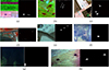 |
Fig. 1 Pseudocolor image (left) and ground-truth image (right). (a) Gulfport. (b) Texas Coast. (c) San Diego-II. (d) HYDICE. (e) San Diego-I. (f) Cement Street. (g) Holly. (h) Jungle. |
3.2 Evaluation metrics
This section mainly introduces how to evaluate the degree of spatial information preservation before and after dimensionality reduction of hyperspectral data, and its impact on object detection tasks. Evaluating the degree of preservation of spatial information before and after dimensionality reduction is equivalent to assessing their spatial structural differences. In this paper, Structure Similarity Index Measure (SSIM), Peak Signal to Noise Ratio (PSNR), and Grey Level Co-occurrence Matrix (GLCM) are used for evaluation. Average the two hyperspectral images before and after dimensionality reduction along the spectral dimension to obtain  , and the SSIM calculation equation between them is
![Mathematical equation: $$ \mathrm{SSIM}\left(\mathbf{X},\mathbf{Z}\right)=\frac{4\overline{\mathbf{X}}\overline{\mathbf{Z}}\mathrm{cov}\left(\mathbf{X},\mathbf{Z}\right)}{\left({\overline{\mathbf{X}}}^2+{\overline{\mathbf{Z}}}^2\right)\left[\mathrm{var}\left(\mathbf{X}\right)+\mathrm{var}\left(\mathbf{Z}\right)\right]}. $$](/articles/jeos/full_html/2025/02/jeos20250029/jeos20250029-eq48.gif) (18)
(18)
SSIM can evaluate the brightness, contrast, and structural differences between two images. It is a perceptual model that is more in line with the intuitive perception of the human eye. The larger the value of SSIM, the more similar the two images are.
PSNR is often used in the field of image compression to evaluate the quality of signal reconstruction, which can characterize the error between corresponding pixels in two images. The larger its value, the more similar the two images are, and its calculation equation is (19)
(19)
Among them, MAX = max(X), ![Mathematical equation: $ \mathrm{MSE}\left(\mathbf{X},\mathbf{Z}\right)=\frac{1}{{mn}}\sum_{i=0}^{m-1}\sum_{j=0}^{n-1}{\left[\mathbf{X}\left(i,\enspace j\right)-\mathbf{Z}\left(i,\enspace j\right)\right]}^2$](/articles/jeos/full_html/2025/02/jeos20250029/jeos20250029-eq50.gif) .
.
Applying GLCM to evaluate the similarity between two images requires separately calculating the feature quantities of the images. The GLCM of a single image is obtained by the following equation:![Mathematical equation: $$ G\left(i,j\right)=\sum_{x=l}^m\sum_{y=l}^n\delta \left[\mathbf{X}\left(i,\enspace j\right)=i\right]\delta \left[\mathbf{X}\left({x}^\mathrm{\prime},\enspace {y}^\mathrm{\prime}\right)=j\right]. $$](/articles/jeos/full_html/2025/02/jeos20250029/jeos20250029-eq51.gif) (20)
(20)
Among them, (x′, y′) = (x + d cosθ, y + d sinθ), d is the distance, θ is the direction. δ is the indicator function, and if the condition holds, it is 1; otherwise, it is 0.
The feature quantities of the gray level co-occurrence matrix G are (21)
(21)
 (22)
(22)
The closer the feature quantity is, the more similar the spatial structure of the image before and after dimensionality reduction. SSIM and PSNR are suitable for evaluating the overall similarity of images. SSIM conforms to human visual perception, while PSNR is used to quantify pixel level differences. GLCM is suitable for texture analysis and can reflect local texture feature differences in images.
The effect of dimensionality reduction can also be demonstrated by downstream object detection tasks. Hyperspectral target detection results are divided into objective and subjective analysis. Subjective analysis mainly involves decision-makers visualizing the detection results by combining ground-truth maps. Objective analysis uses receiver operating characteristic (ROC) and area under the curve (AUC). The ROC curve establishes the correlation between false alarm probability (PFA) and detection probability (PD) based on a common threshold τ. The traditional two-dimensional ROC curve mainly comprises the τ – PFA relationship curve and the τ – PD relationship curve. The definitions of PD and PFA are as follows: (23)
(23)
Where N d is the number of real target pixels detected, which is the number of pixels that belong to the target and are considered the target by the detector, N t represents the total number of target pixels in the image. N f represents the number of detected false alarm pixels that belong to the background but are considered targets by the detector. N b represents the total number of background pixels in the image.
AUC quantitatively describes the degree of deviation of the ROC curve from the upper left corner. The values are as follows: (24)
(24)
The greater the offset of the ROC curve to the upper left, the larger the area below the curve line and the larger the AUC, indicating better detection performance. The flatter the ROC curve, the smaller the area below the curve, and the smaller the AUC, the worse the detection effect.
3.3 Parameter sensitivity analysis
Acquiring an accurate noise covariance matrix is a critical task, as its precision directly impacts the performance of the proposed method. Common approaches for estimating the noise covariance matrix include the median filtering method [30], spectral and spatial de-correlation (SSDC) method [31], HySime method [32], and Per-Pixel method [33]. These methods provide pixel-by-pixel noise estimation for hyperspectral data and facilitate the calculation of the noise covariance matrix. This section investigates the performance differences of the proposed method when using four distinct noise matrices as inputs and evaluates the role of the spatial information preservation term. Figure 2 illustrates the spatial information preservation effects of the proposed method and MNF under the four noise estimation methods. The results represent the average values obtained from experiments conducted on eight hyperspectral datasets. Under the metrics of SSIM, PSNR, and GLCM Contrast, the noise matrix provided by the SSDC method enables the proposed method to achieve optimal performance. Additionally, it demonstrates competitive performance under the GLCM Correlation metric. It is evident that the proposed method consistently outperforms the standard MNF across all metrics, highlighting the significant contribution of the spatial information preservation term.
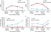 |
Fig. 2 The spatial information preservation effect of the proposed method and the MNF method under four noise estimation methods. (a) SSIM. (b) PSNR. (c) GLCM Contrast. (d) GLCM Correlation. |
The impact of different noise inputs on target detection after dimensionality reduction will also be examined. The following target detection methods will be used for the reduced dimensional data:
-
Two-Step Generalized Likelihood Ratio Test (2S-GLRT) [34]: A hyperspectral anomaly detection method for Gaussian backgrounds with unknown covariance matrices. Adaptive detector based on generalized likelihood ratio testing.
-
Spectral Match Filter (SMF) [35]: The derivation of the decision function using the correlation matrix or covariance matrix information of the tested image is based on probability and statistical theory.
-
Adaptive Cosine Estimation (ACE) [36]: Estimation of unknown signal covariance structure and level based on training data sample covariance, used for detecting target signals in noise.
-
Hybrid Structured Detector (HUD) [37]: Based on the use of physically meaningful linear mixing models and statistical hypothesis testing, the background is modeled as a multivariate normal distribution, and the known physical properties of the problem are explained by the physical endmembers and abundance.
-
Robust Graph Autoencoders (RGAE) [38]: Robust anomaly detector based on autoencoder framework. Embedding a superpixel segmentation graph regularization term in autoencoder to maintain geometric structure and local spatial consistency can reduce search space.
-
Autonomous Hyperspectral Anomaly Detection (Auto-AD) [39]: A fully convolutional autoencoder framework with skip connections can effectively detect targets by reducing the weight of abnormal pixels during the reconstruction process through an adaptive weighted loss function.
The methods related to deep learning are implemented on Ubuntu systems with PyTorch 1.8 and Python 3.8, including two GeForce RTX 2080 GPUs. Other methods are implemented on the Windows system using MATLAB R2023b, with a CPU of i7-11800H and a GPU of GeForce GRX 3050Laptop. The detection results before and after dimensionality reduction using various methods are shown in Figure 3–10. From the perspective of noise estimation methods, the dimensionality reduced data obtained by applying the Median filtering method brings many false alarms to detection, making it difficult to accurately distinguish between targets and backgrounds regardless of the detection method used. The simple principle and method of Median filtering result in poor accuracy of noise estimation, misleading the dimensionality reduction process and potentially causing the transformed data to contain a large amount of noise, leading to ineffective differentiation between targets and backgrounds during detection. SSDC, the per-pixel method, and Hyres all consider spectral correlation, and their noise estimation accuracy has been validated in previous studies [31–33]. The best performance is achieved when dimensionality reduction is performed using SSDC and the per-pixel method. SMF and ACE have better detection performance on private datasets. In tests on public datasets, HUD and RGAE performed well. From the detection result graph, it can be seen that 2S-GLRT has a low detection rate for all data, making it difficult to identify targets regardless of whether dimensionality reduction is performed. Table 1 shows the average AUC values of different detection methods across all datasets. From the table, it can be seen that dimensionality reduction has little overall impact on detection accuracy. When using only the Per-Pixel method as the noise estimation method, there is an increase, and when applying other methods, there is a slight decrease, but it is within an acceptable range. The average AUC value before dimensionality reduction was 0.8573, and the average AUC value after dimensionality reduction was 0.8537, a decrease of 0.42%. Figure 11 shows the ROC curves of detection results for different data and detection methods before and after dimensionality reduction (the detection performance of 2S-GLRT is too poor regardless of dimensionality reduction, so it is not shown). Per-Pixel method is used as the noise estimation method. The ROC curve and score plot of the detection results both indicate that dimensionality reduction increases the detection score of the target while enhancing the generation of false alarms.
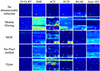 |
Fig. 3 Detection results on the Gulfport dataset. |
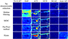 |
Fig. 4 Detection results on the HYDICE dataset. |
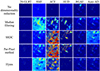 |
Fig. 5 Detection results on the Texas Coast dataset. |
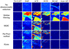 |
Fig. 6 Detection results on the San Diego-I dataset. |
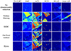 |
Fig. 7 Detection results on the San Diego-II dataset. |
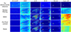 |
Fig. 8 Detection results on the Cement Street dataset. |
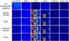 |
Fig. 9 Detection results on the Holly dataset. |
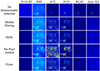 |
Fig. 10 Detection results on the Jungle dataset. |
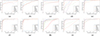 |
Fig. 11 ROC curve of detection results. Before dimensionality reduction: (a)SMF. (b) ACE. (c) HUD. (d) RGAE. (e) Auto-AD. After dimensionality reduction: (f) SMF. (g) ACE. (h) HUD. (i) RGAE. (j) Auto-AD. |
Average AUC values of different detection methods on all datasets.
Another factor worth considering is the impact of noise estimation methods on the overall dimensionality reduction time. Table 2 shows the running time of the dimensionality reduction process under different noise estimation methods across various datasets, representing the average time after ten independent runs. The Median filtering method takes the shortest time due to its simplicity and efficient computational approach. In contrast, the Per-Pixel method has a running time that is an order of magnitude higher than the other three methods, resulting in a significant increase in computational cost. The size of the dataset also significantly impacts the running time of dimensionality reduction methods, with larger datasets generally requiring longer processing times. Figure 12 demonstrates that the running time scales linearly with the data volume.
 |
Fig. 12 Relationship between runtime and data volume. (a) Median filtering. (b) SSDC. (c) MR method. (d) Hyres. |
The running time of dimensionality reduction.
3.4 The impact on spatial information
This section will discuss the effectiveness of the proposed method in preserving spatial information and compare it with some unsupervised dimensionality reduction methods. Including PCA [8], MNF [14], Superpixelwise Unsupervised Linear Discriminant Analysis (SuperULDA) [40], Laplacian Regularized Collaborative Representation Projection (LRCRP) [41], Superpixelwise Principal Component Analysis (SuperPCA) [42], and Dual Graph Autoencoder (DGAE) [43]. All experiments were conducted on the eight data points mentioned earlier, and the experimental results were averaged. The results of the proposed method are based on the average values of the four noise matrices mentioned above as inputs.
Table 3 demonstrates the effectiveness of various dimensionality reduction methods in preserving spatial information. Overall, the proposed method performs well in all indicators and has a leading advantage. Among them, the proposed method achieved the best performance in SSIM, GLCM Contrast, and GLCM Correlation. In terms of PSNR, the proposed method is second only to SuperPCA, indicating that the proposed method has good spatial preservation effects on the overall structure and some prominent textures. An obvious phenomenon is that MNF performs the worst in SSIM, GLCM Contrast, and GLCM Correlation, and only outperforms LRCRP in PSNR. The possible reason is that MNF only focuses on improving the signal-to-noise ratio, while the dimensionality reduction mechanisms of other algorithms contain limitations on the overall pixel variation. This indicates that the spatial information preservation term added by the proposed method has a good effect on preserving spatial information.
The spatial information retention effect of various dimensionality reduction methods.
3.5 The impact on the accuracy of target detection
This section discusses the performance of the proposed method and comparative dimensionality reduction methods in target detection. The comparative methods and target detection methods are selected as mentioned above. Figures 13–20 illustrate the detection performance of various dimensionality reduction methods across eight datasets using different detection methods. For the San Diego-I dataset, the image obtained after dimensionality reduction via SuperPCA resulted in singular values when detected by HUD, leading to detection results filled with zeros. In the Jungle dataset, the image processed by SuperPCA contained Not-a-Number (NaN) values, rendering detection impossible. The DGAE method involves an array with a size quadratic to the number of spatial pixels during dimensionality reduction. Due to the large spatial dimensions of the Cement Street dataset, Holly dataset, and Jungle dataset, the memory required to run the DGAE dimensionality reduction code exceeded capacity, preventing the experiments from being conducted. Additionally, an error occurred during the superpixel segmentation step of SuperULDA dimensionality reduction on the Jungle dataset, resulting in no dimensionality reduction output. From a subjective evaluation of the detection results, SuperPCA, SuperULDA, and DGAE methods performed poorly on most datasets, exhibiting a significant number of false alarms and chaotic detection outcomes. PCA and MNF methods showed fewer false alarms but also had lower detection rates. The proposed method and the LRCRP method performed relatively well, accurately detecting targets in some datasets, though they exhibited higher false alarms in others. Supervised detection methods generally provided results with higher false alarms, while unsupervised detection methods tended to yield lower detection rates. Table 4 presents the objective evaluation metrics, specifically the AUC values of detection results for different dimensionality reduction methods under various detection methods. The proposed method achieved the best performance in four out of the six detection methods and demonstrated the highest average detection performance, proving that the proposed dimensionality reduction method effectively supports downstream tasks.
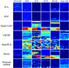 |
Fig. 13 Detection results on the Gulfport dataset. |
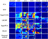 |
Fig. 14 Detection results on the HYDICE dataset. |
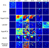 |
Fig. 15 Detection results on the Texas Coast dataset. |
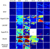 |
Fig. 16 Detection results on the San Diego-I dataset. |
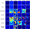 |
Fig. 17 Detection results on the San Diego-II dataset. |
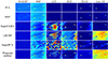 |
Fig. 18 Detection results on the Cement Street dataset. |
 |
Fig. 19 Detection results on the Holly dataset. |
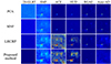 |
Fig. 20 Detection results on the Jungle dataset. |
The average AUC values of different detection methods under different dimensionality reduction methods.
3.5 The impact on time consumption
This section will examine the impact of dimensionality reduction on the running time of detection methods. Figure 21 shows the variation of running time under different detection methods, with the y-axis representing the ratio of running time after dimensionality reduction to running time before dimensionality reduction. From the graph, it can be seen that dimensionality reduction has a significant effect on reducing the running time of most detection methods, especially 2S-GLRT, SMF, and ACE. Due to its characteristics, the HUD method does not have a very significant effect on reducing runtime. The time reduction effect of Auto-AD method on public datasets is poor.
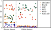 |
Fig. 21 Changes in running time under different detection methods. |
4 Conclusion
This paper proposes a dimensionality reduction method based on spatial-spectral preservation and minimum noise fraction. The method consists of two parts: linear transformation and selection strategy. The linear transformation aims to maximize the signal-to-noise ratio and image structural similarity, preserving spatial information while eliminating noise effects. The selection strategy considers the relative position of each pixel in the feature space and selects the component group with the smallest average change in relative position as the final result of dimensionality reduction. Experiments show that the accuracy of noise estimation significantly impacts the proposed method. It is necessary to consider the accuracy of noise estimation and balance its computational time to improve timeliness. The proposed method effectively preserves both spatial and spectral information of the data, enabling target detection methods to demonstrate their effectiveness and outperform comparative approaches. For most target detection methods, dimensionality reduction can significantly enhance their timeliness. It should be noted that the proposed method only uses target detection as a downstream task for validation, which presents certain limitations.
Funding
This research did not receive any specific funding.
Conflicts of interest
The authors declare that they have no competing interests to report.
Data availability statement
Some hyperspectral images used in this paper are public data sets commonly used in the field, which can be obtained from the Internet according to the description of the data set in this paper. The remaining dataset was taken by the author themselves and can be obtained or inquired about through email.
Author contribution statement
All authors have reviewed, discussed, and agreed to their personal contributions. The specific situation is as follows: Conceptualization, Bing Zhou; Methodology, Algorithms, and Writing, Lei Deng; Experimental verification, Jiaju Ying; Analysis, Qianghui Wang; Data visualization and Review, Yue Cheng.
References
- El Abady NF, Zayed HH, Taha M, An efficient technique for detecting document forgery in hyperspectral document images, Alexandria Eng. J. 85, 207–217 (2023). https://doi.org/10.1016/j.aej.2023.11.040. [Google Scholar]
- Tuya, Graph convolutional enhanced discriminative broad learning system for hyperspectral image classification, IEEE Access 10, 90299–90311 (2022). https://doi.org/10.1109/ACCESS.2022.3201537. [Google Scholar]
- Ma F, Liu SY, Yang FX, Xu GX, Piecewise weighted smoothing regularization in tight framelet domain for hyperspectral image restoration, IEEE Access 11, 1955–1969 (2023). https://doi.org/10.1109/ACCESS.2022.3233831. [Google Scholar]
- Yuen PWT, Richardson M, An introduction to hyperspectral imaging and its application for security, surveillance and target acquisition, Imaging Sci. J. 58, 241–253 (2010). https://doi.org/10.1179/174313110X12771950995716. [Google Scholar]
- Lv WJ, Wang XF, Overview of hyperspectral image classification, J. Sens. 2020, 4817234 (2020). https://doi.org/10.1155/2020/4817234. [Google Scholar]
- Uddin MP, Manun MA, Hossain MA, PCA-based feature reduction for hyperspectral remote sensing image classification, IETE Tech Rev 38, 377–396 (2021). https://doi.org/10.1080/02564602.2020.1740615. [Google Scholar]
- Islam MT, Islam MR, Uddin MP, Ulhaq A, A deep learning-based hyperspectral object classification approach via imbalanced training samples handling, Remote Sens. 15, 3532 (2023). https://doi.org/10.3390/rs15143532. [Google Scholar]
- Rodarmel C, Shan J, Principal component analysis for hyperspectral image classification, Surv. Land Inf. Sci. 62, 115–122 (2002). [Google Scholar]
- Du Q, Chang CI, Segmented PCA-based compression for hyperspectral image analysis, in Proceedings of the Chemical and Biological Standoff Detection, Vol. 5268 (SPIE, Bellingham, WA, USA, 2004), 274–281. https://doi.org/10.1117/12.518835. [Google Scholar]
- Hyvärinen EOA, Karhunen J. Independent Component Analysis (Wiley, Hoboken NJ, 2001). ISBN:9780471221319. https://doi.org/10.1002/0471221317. [Google Scholar]
- Bakken S, Orlandic M, Johansen TA, The effect of dimensionality reduction on signature-based target detection for hyperspectral imaging, SPIE Opt. Eng. Appl. 111310L (2019). https://doi.org/10.1117/12.2529141. [Google Scholar]
- Falco N, Bruzzone L, Benediktsson JA, An ICA based approach to hyperspectral image feature reduction, Proc. IEEE Geosci. Remote Sens. Symp., 3470–3473 (2014). https://doi.org/10.1109/IGARSS.2014.6947229. [Google Scholar]
- Zhang ZY, Data Mining Found, in: Intell Paradig, 1st edn., edited by Holmes DE, Lakshmi C (Springer-Verlag, Berlin, Heidelberg, 2012). ISBN: 978-3-642-23241-1. [Google Scholar]
- Chen G, Qian SE, Evaluation and comparison of dimensionality reduction methods and band selection, Can J Remote Sens 34, 26–36 (2008). https://doi.org/10.5589/m08-007. [Google Scholar]
- Guan LX, Xie WX, Pei JH, Segmented minimum noise fraction transformation for efficient feature extraction of hyperspectral images, Pattern Recognit 48, 3216–3226 (2015). https://doi.org/10.1016/j.patcog.2015.04.013. [Google Scholar]
- Groves P, Bajcsy P, Methodology for hyperspectral band and classification model selection, in: IEEE Workshop on Advances in Techniques for Analysis of Remotely Sensed Data (IEEE, Greenbelt, MD, 2003), pp. 120–128. https://doi.org/10.1109/WARSD.2003.1295183. [Google Scholar]
- Du Q, Yang H, Similarity-based unsupervised band selection for hyperspectral image analysis, IEEE Geosci. Remote Sens. Lett. 5(4, 564–568 (2008). https://doi.org/10.1109/LGRS.2008.2000619.. [Google Scholar]
- Su HJ, Sheng YH, Yang H, Du Q, Orthogonal projection divergence-based hyperspectral band selection, Spectroscopy Spectral Anal. 31(5), 1309–1313 (2011). https://doi.org/10.3964/j.issn.1000-0593(2011)05-1309-05. [Google Scholar]
- Su HJ, Du Q, Hyperspectral band clustering and band selection for urban land cover classification, Geocarto Int. 27(5), 395–411 (2012). https://doi.org/10.1080/10106049.2011.643322.. [Google Scholar]
- Sun WW, Zhang LP, Du B, Li WY, Mark Lai Y, Band selection using improved sparse subspace clustering for hyperspectral imagery classification, IEEE J. Sel. Top. Appl. Earth Obs. Remote Sens. 8(6), 2784–2797 (2015). https://doi.org/10.1109/JSTARS.2015.2417156. [Google Scholar]
- Sun WW, Peng JT, Yang G, Du Q, Correntropy-based sparse spectral clustering for hyperspectral band selection, IEEE Geosci. Remote Sens. Lett. 17(3), 484–488 (2020). https://doi.org/10.1109/LGRS.2019.2924934. [Google Scholar]
- Zhu B, Jin Y, Guan XH, Dong YN, SSMM: Semi-supervised manifold method with spatial-spectral self-training and regularized metric constraints for hyperspectral image dimensionality reduction, Int. J. Appl. Earth Obs. Geoinform. 136, 104373 (2025). https://doi.org/10.1016/j.jag.2025.104373. [Google Scholar]
- Du PJ, Wang XM, Tan K, Xia JS, Dimensionality reduction and feature extraction from hyperspectral remote sensing imagery based on manifold learning, Geomat. Inform. Sci Wuhan Univ 36(2), 148–152 (2011). [Google Scholar]
- Fang Y, Li H, Ma Y, Liang K, Hu YJ, Zhang SJ, Wang HY, Dimensionality reduction of hyperspectral images based on robust spatial information using locally linear embedding, IEEE Geosci. Remote Sens. Lett. 11(10), 1712–1716 (2014). https://doi.org/10.1109/LGRS.2014.2306689. [Google Scholar]
- Huang H, Shi GY, Duan YL, Zhang LM, Dimensionality reduction method for hyperspectral images based on weighted spatial-spectral combined preserving embedding, Acta Geod. Cartogr. Sin. 48(8), 1014–1024 (2019). [Google Scholar]
- Wang JL, Hou B, Jiao LC, Wang S, POL-SAR image classification based on modified stacked autoencoder network and data distribution, IEEE Trans. Geosci. Remote Sens. 58(3), 1678–1695 (2020). https://doi.org/10.1109/TGRS.2019.2947633. [Google Scholar]
- Tao C, Pan HB, Li YS, Zou ZR, Unsupervised spectral-spatial feature learning with stacked sparse autoencoder for hyperspectral imagery classification, IEEE Geosci. Remote Sens. Lett. 12(12), 2438–2442 (2015). https://doi.org/10.1109/LGRS.2015.2482520. [Google Scholar]
- Zhang MY, Gong MG, Mao YS, Li J, Wu Y, Unsupervised feature extraction in hyperspectral images based on Wasserstein generative adversarial network, IEEE Trans. Geosci. Remote Sens. 57(5), 2669–2688 (2019). https://doi.org/10.1109/TGRS.2018.2876123. [Google Scholar]
- Su HJ, Wu ZY, Zhang HH, Du Q, Hyperspectral anomaly detection: a survey, IEEE Geosci. Remote Sens. Mag. 10(1), 64–90 (2022). https://doi.org/10.1109/MGRS.2021.3105440. [Google Scholar]
- Tong QX, Zhang B, Zhen LF, Hyperspectral Remote Sensing: principles, techniques, and applications, edited by Chen ZX, 1st edn. (Higher Education Press, Beijing, 2006). [Google Scholar]
- Roger RE, Arnold JF, Reliably estimating the noise in AVIRIS hyperspectral images, Int. J. Remote Sens. 17, 1951–1962 (1996). https://doi.org/10.1080/01431169608948750. [Google Scholar]
- Rasti B, Ulfarsson MO, Ghamisi P, Automatic hyperspectral image restoration using sparse and low-rank modeling, IEEE Geosci Remote Sens Lett 14, 2335–2339 (2017). https://doi.org/10.1109/LGRS.2017.2764059. [Google Scholar]
- Mahmood A, Sears M, Per-pixel noise estimation in hyperspectral images, IEEE Geosci. Remote Sens. Lett. 19, 5503205 (2022). https://doi.org/10.1109/LGRS.2021.3064998. [Google Scholar]
- Liu J, Hou Z, Li W, Tao R, Orlando D, Li H, Multipixel anomaly detection with unknown patterns for hyperspectral imagery, IEEE Trans. Neural Netw. Learn. Syst. 33, 5557–5567 (2022). https://doi.org/10.1109/TNNLS.2021.3071026. [Google Scholar]
- Manolakis D, Lockwood R, Cooley T, Is there a best hyperspectral detection algorithm, Proc. SPIE 7334, 733402 (2009). https://doi.org/10.1117/12.816917. [Google Scholar]
- Kraut S, Scharf L, The CFAR adaptive subspace detector is a scale-invariant GLRT, IEEE Trans. Signal Process 47, 2538–2541 (1999). https://doi.org/10.1109/SSAP.1998.739333. [Google Scholar]
- Broadwater J, Chellappa R, Hybrid detectors for subpixel targets, IEEE Trans. Pattern Anal. Mach. Intell. 29, 1891–1903 (2007). https://doi.org/10.1109/TPAMI.2007.1104. [Google Scholar]
- Fan G, Ma Y, Mei X, Fan F, Huang J, Ma J, Hyperspectral anomaly detection with robust graph autoencoders, IEEE Trans. Geosci. Remote Sens. 60, 1–14 (2022). https://doi.org/10.1109/TGRS.2021.3097097. [CrossRef] [Google Scholar]
- Wang S, Wang X, Zhang L, Zhong Y, Auto-AD: Autonomous hyperspectral anomaly detection network based on fully convolutional autoencoder, IEEE Trans Geosci Remote Sens 60, 1–14 (2022). https://doi.org/10.1109/TGRS.2021.3057721. [CrossRef] [Google Scholar]
- Lu P, Jiang XW, Zhang YS, Liu XB, Cai ZH, Jiang JJ, Plaza A, Spectral–spatial and superpixelwise unsupervised linear discriminant analysis for feature extraction and classification of hyperspectral images, IEEE Trans. Geosci. Remote Sens. 61, 1–15 (2023). https://doi.org/10.1109/TGRS.2023.3330474. [Google Scholar]
- Jiang X, Xiong L, Yan Q, Zhang Y, Liu X, Cai Z, Unsupervised dimensionality reduction for hyperspectral imagery via Laplacian regularized collaborative representation projection, IEEE Geosci. Remote Sens. Lett. 19, 1–5 (2022). https://doi.org/10.1109/LGRS.2022.3153041. [CrossRef] [Google Scholar]
- Jiang J, Ma J, Chen C, Wang Z, Cai Z, Wang L, SuperPCA: A superpixelwise PCA approach for unsupervised feature extraction of hyperspectral imagery, IEEE Trans. Geosci. Remote Sens. 56(8), 4581–4593 (2018). https://doi.org/10.1109/TGRS.2018.2828029. [Google Scholar]
- Zhang Y, Wang Y, Chen X, Jiang X, Zhou Y, Spectral–spatial feature extraction with dual graph autoencoder for hyperspectral image clustering, IEEE Trans. Circuit.Syst. Video Technol. 32(12), 8500–8511 (2022). https://doi.org/10.1109/TCSVT.2022.3196679. [Google Scholar]
All Tables
The spatial information retention effect of various dimensionality reduction methods.
The average AUC values of different detection methods under different dimensionality reduction methods.
All Figures
|
Fig. 1 Pseudocolor image (left) and ground-truth image (right). (a) Gulfport. (b) Texas Coast. (c) San Diego-II. (d) HYDICE. (e) San Diego-I. (f) Cement Street. (g) Holly. (h) Jungle. |
| In the text | |
|
Fig. 2 The spatial information preservation effect of the proposed method and the MNF method under four noise estimation methods. (a) SSIM. (b) PSNR. (c) GLCM Contrast. (d) GLCM Correlation. |
| In the text | |
|
Fig. 3 Detection results on the Gulfport dataset. |
| In the text | |
|
Fig. 4 Detection results on the HYDICE dataset. |
| In the text | |
|
Fig. 5 Detection results on the Texas Coast dataset. |
| In the text | |
|
Fig. 6 Detection results on the San Diego-I dataset. |
| In the text | |
|
Fig. 7 Detection results on the San Diego-II dataset. |
| In the text | |
|
Fig. 8 Detection results on the Cement Street dataset. |
| In the text | |
|
Fig. 9 Detection results on the Holly dataset. |
| In the text | |
|
Fig. 10 Detection results on the Jungle dataset. |
| In the text | |
|
Fig. 11 ROC curve of detection results. Before dimensionality reduction: (a)SMF. (b) ACE. (c) HUD. (d) RGAE. (e) Auto-AD. After dimensionality reduction: (f) SMF. (g) ACE. (h) HUD. (i) RGAE. (j) Auto-AD. |
| In the text | |
|
Fig. 12 Relationship between runtime and data volume. (a) Median filtering. (b) SSDC. (c) MR method. (d) Hyres. |
| In the text | |
|
Fig. 13 Detection results on the Gulfport dataset. |
| In the text | |
|
Fig. 14 Detection results on the HYDICE dataset. |
| In the text | |
|
Fig. 15 Detection results on the Texas Coast dataset. |
| In the text | |
|
Fig. 16 Detection results on the San Diego-I dataset. |
| In the text | |
|
Fig. 17 Detection results on the San Diego-II dataset. |
| In the text | |
|
Fig. 18 Detection results on the Cement Street dataset. |
| In the text | |
|
Fig. 19 Detection results on the Holly dataset. |
| In the text | |
|
Fig. 20 Detection results on the Jungle dataset. |
| In the text | |
|
Fig. 21 Changes in running time under different detection methods. |
| In the text | |
Current usage metrics show cumulative count of Article Views (full-text article views including HTML views, PDF and ePub downloads, according to the available data) and Abstracts Views on Vision4Press platform.
Data correspond to usage on the plateform after 2015. The current usage metrics is available 48-96 hours after online publication and is updated daily on week days.
Initial download of the metrics may take a while.