| Issue |
J. Eur. Opt. Society-Rapid Publ.
Volume 22, Number 1, 2026
|
|
|---|---|---|
| Article Number | 6 | |
| Number of page(s) | 14 | |
| DOI | https://doi.org/10.1051/jeos/2026001 | |
| Published online | 11 February 2026 | |
Research Article
Underwater 3D target detection: Semi-analytic Monte Carlo model and UAV-based scanning lidar system
1
Aerospace Laser Technology and System Department, Shanghai Institute of Optics and Fine Mechanics, Chinese Academy of Sciences, Shanghai 201800, PR China
2
Center of Materials Science and Optoelectronics Engineering, University of Chinese Academy of Sciences, Beijing 100049, PR China
3
Wangzhijiang Innovation Center for Laser, Aerospace Laser Technology and System Department, Shanghai Institute of Optics and Fine Mechanics, Chinese Academy of Sciences, Shanghai 201800, PR China
4
School of Physical Science and Technology, Shanghai Tech University, Shanghai 201210, PR China
5
Naval Research Institute, Tianjin 300061, PR China
6
Laoshan Laboratory, Qingdao 266237, PR China
* Corresponding author: This email address is being protected from spambots. You need JavaScript enabled to view it.
Received:
26
November
2025
Accepted:
3
January
2026
Abstract
Lidar has been widely applied in marine research due to its strong penetration capability in water. To study the lidar detection of underwater targets, a semi-Monte Carlo model of target detection (MCT) is developed to simulate the scanning signals, incorporating three-dimensional interaction processes between the beam and the target, the wind-driven surface waves and stratified water columns. A UAV-based linear scanning oceanic lidar system (SOL) is developed for model validation. The model is validated by the lidar equation results with a less than 5% mean relative error within the upper 50 m, and further confirmed by the SOL field experiments through consistent target localization. The detection capabilities of SOL are analyzed based on the MCT model for Jerlov II and Jerlov 3C water types, and an extended detection range is introduced to evaluate the variation of horizontal scanning resolution with target depth, providing guidance for balancing detection capability and efficiency under varying conditions.
Key words: Lidar application / Monte Carlo method / UAV-based lidar / Underwater target detection
© The Author(s), published by EDP Sciences, 2026
 This is an Open Access article distributed under the terms of the Creative Commons Attribution License (https://creativecommons.org/licenses/by/4.0), which permits unrestricted use, distribution, and reproduction in any medium, provided the original work is properly cited.
1 Introduction
Ocean plays a vital role in regulating the global climate, sustaining biodiversity, and supporting essential resource [1–3]. Ocean sensing is therefore a fundamental prerequisite for understanding and sustainably utilizing the ocean. However, conventional detection methods face intrinsic limitations: sonar systems aren’t able to detect through air–water interface, while passive satellite remote sensing is not able to provide the vertical information on the upper ocean layers [4–7]. Among ocean sensing techniques, Light Detection and Ranging (Lidar) has emerged as an effective alternative. As an active remote sensing system, lidar penetrates the air–water interface and captures high spatial and temporal resolution profiles of subsurface structures [8–10]. These capabilities establish lidar as an essential complement to existing ocean sensing approaches.
Lidars has been developed for diverse applications, among which one of the earliest and most prominent uses is topobathymetry [11]. Modern topobathymetry lidar systems are capable of achieving high-precision integrated coastal and terrestrial topographic mapping [12–15], seabed substrate classification [10, 16], as well as surveying in turbid waters and shallow areas [17]. Moreover, lidar profiling information provides essential support for studying marine organisms and retrieving seawater optical properties. Investigating the distribution and dynamics of phytoplankton [18–22] based on lidar profiling data contributes to a deeper understanding of the mechanisms driving marine primary productivity and the global carbon cycle. Lidar has also been proven to be highly effective in surveying fishery resources [23–27] near the sea surface, and its performance on deriving optical properties [28–32], such as the attenuation coefficient and volume backscattering, has been validated by shipborne in-situ measurements. Additionally, lidar enables measurements of wave characteristics without contacting the water body or disturbing hydrodynamic processes, serving as an effective tool for observing ocean surface waves [33, 34] and internal waves [35, 36].
Underwater target detection is now emerging as a new direction for lidar applications, which has importance influences on human activities, such as navigation planning and port construction [2, 23]. In the field of underwater target detection, current research mainly focuses on two directions: underwater imaging and rapid detection of underwater targets. Since the first application of single-photon avalanche diode (SPAD) arrays to underwater imaging is represented, single-photon imaging technology has steadily advanced [37]. Subsequently, the first fully submerged underwater lidar transceiver system based on single-photon detection technologies has been demonstrated, achieving images of stationary targets at ranges up to 7.5 attenuation lengths [38]. More recently, a compact, all-fiber underwater imaging lidar has been presented that achieved imaging distances exceeding 10 times the optical attenuation length, further highlighting the progress in underwater imaging lidar research [39]. However, the application of lidar for rapidly detecting underwater targets from above water surface remains limited. Only some mapping lidar systems possess the capability for rapid target detection, and there is no dedicated lidar system specifically designed for this purpose. The underwater obstruction detection capabilities of the Scanning Hydrographic Operational Airborne Lidar Survey (SHOALS) were discussed by adopting the enhanced object detection algorithm [12, 13, 40]. A lightweight UAV-borne lidar Mapper4000 U was developed for shallow water mapping, which had the ability to recognize the existence of a 1-m cube and the rough shape of a 2-m cube at a depth of 12 m by point cloud fitting [41].
There is also a great deal of algorithms to generate lidar signals, such as the lidar equation, analytical model and Monte Carlo simulation technique. The lidar equation is able to describe depth-dependent lidar signals quickly but has limitations in dealing with multiple scattering [42, 43]. The analytical model is highly difficult to solve due to its complexity. Only approximate solutions can be achieved through some idealized assumption [44]. The standard Monte Carlo method is based on a huge number of random calculations of photons’ movements in the water, and photons can be accepted only when they finally arrive at the receiver aperture. The condition is too strict to reconstruct the lidar profiles, consuming a large amount of computing power and time [45]. The semi-analytic Monte Carlo radiative transfer model for oceanographic lidar systems (SALMON) is based on the method of stochastic and analytic techniques, which estimates the contribution of each scattered photon by the function from a particle scattering position to the detector [46]. With the advantages in computational efficiency and accuracy, the SALMON model has been the foundation of the MC simulator for oceanic lidar. After decades of development, the semi-analytical MC model has been applied in seabed mapping, retrievals of bio-optical properties and polarized signal analysis and so on [47–52]. However, current research in ocean mapping or target detection is primarily focused on the seabed modeling and has some overly idealized assumptions, which assumes that the seabed fills the entire lidar field of view and simplifies the photon–seabed interactions, without accounting for three-dimensional interactions or the blocking effect on the beam transmission [53, 54]. Besides, the majority of these studies assume a homogeneous water body and neglect environmental noises, making it difficult to capture the complexity of realistic detection scenarios. On the other hand, the simulators for oceanic lidar profiling have made some advancements in accuracy. While these simulators mainly focus on the slope variations of lidar returns that are closely related to signal retrieval, photon propagation only needs to account for the effects of absorption and scattering by the water, which makes them incapable of detecting three-dimensional target.
As it stands, lidar systems that are applicable to or specifically designed for underwater target detection have yet to be widely developed. A dedicated Monte Carlo simulator for three-dimensional underwater target detection has yet to be established. Three-dimensional simulations are crucial for capturing spatial heterogeneity, beam divergence, and realistic scanning geometries. Therefore, it is highly necessary to develop a simulator that not only emphasizes accuracy but also generates three-dimensional target detection as well as a lidar system designed base on the simulator’s guidance.
Our research group has already conducted extensive prior work in this area. A standard MC model to detect infinite planar target [55] and a semi-analytical MC model to detect a two-dimensional flat plane with limited size [56] have been proposed. In this paper, we present a refined semi-analytical Monte Carlo model for underwater three-dimensional target detection (MCT), especially including the interaction process between the beam and the target, the blocking effect on the beam transmission and the reception of the target reflection signals. The MCT model can simulate the scanning signals for underwater three-dimensional targets through surface waves in stratified water columns, and incorporate realistic environmental noise to better approximate field conditions. We develop a miniaturized, linear scanning oceanic lidar system (SOL) deployable on commercial UAV platforms. The MCT model is validated by comparisons with the lidar equation results and field measurements from SOL. Furthermore, using MCT, we evaluate SOL’s detection capabilities in Jerlov II and Jerlov 3C waters, define an extended detection range metric, and examine its relationship with vertical penetration and horizontal scanning resolution, offering an integrated framework for system performance assessment and design optimization in realistic marine environments.
In the rest of this paper, we present the MCT model in Section 2. We present the SOL system in Section 3. The MCT model is validated in Section 4. The target detection capabilities of SOL in different waters are evaluated in Section 5. The conclusion is made up in Section 6.
2 Monte Carlo model of underwater target detection
For a complete and detailed introduction to the MCT model, a cylinder target is chosen as a representative example. The cylindrical geometry captures essential features relevant to underwater lidar detection, including extended surfaces, well-defined edges, and stable occlusion characteristics under scanning illumination. As a representative intermediate case, the cylindrical geometry combines manageable geometric complexity with physically meaningful target characteristics relevant to practical detection scenarios. It is worth emphasizing that the proposed MCT model is formulated in a geometry-independent manner. Other target can be incorporated by modifying the geometric description.
The main parts are introduced below, and the flow chart of the model is shown in Figure 1. The whole simulation starts with the emission of photons and ends with their final death. During the propagation process, the photon can be scattered, reflected by the target, escaping from the boundary, or received by the detector. The surface of the target is seen as ideal Lambertian. The inherent optical properties (IOPs) model of water used in simulation is based on previous research [43, 57–62].
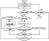 |
Fig. 1 Flow chart of MCT simulation model. |
2.1 Launching
The Cartesian coordinates of the simulation model are shown in Figure 2a, the initial position of the lidar system is Pst
= [xst, yst, 0], and the downward direction of the z-axis is positive. The intensity of the emitted beam follows a Gaussian distribution, and the initial position of the photon is sampled from the laser spot on the water surface (Fig. 2b). The intensity distribution on the water surface is [63] (1)
(1)
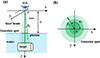 |
Fig. 2 (a) Global coordinate system of the simulation model, and (b) sampling the point from the Gaussian spot. |
where σ is standard deviation of Gaussian distribution. The sampled spot radius RG is expressed as (2)
(2)
where ξrnd is a random number uniformly distributed over (0, 1). The initial azimuth angle on the Gaussian spot is sampled as follow (3)
(3)
The photon’s initial position on the water surface then be obtained as (4)
(4)
where H is the flight height. The lidar system positions xst and yst will be changed with the UAV moves. The initial incident direction of the photon is (5)
(5)
where the emitting angle can be calculated by θ0 ≈ tan−1(RG/H). When the photon passes through the air–sea interface, the instantaneous state of the waves must be taken into account. The normal vector of the surface wave is defined as (6)
(6)
where  is also sampled by equation (3). The normalized probability density function of θw is proposed by Cox and Munk [64]:
![Mathematical equation: $$ \begin{array}{c}p\left({\theta }_w\right)=\frac{2}{{\phi }_w^2}{exp}\left[\frac{-{\mathrm{tan}}^2\left({\theta }_w\right)}{{\sigma }^2}\mathrm{tan}\left({\theta }_w\right){\mathrm{sec}}^2\left({\theta }_w\right)\right],\end{array} $$](/articles/jeos/full_html/2026/01/jeos20250088/jeos20250088-eq8.gif) (7)
(7)
where σ is the root-mean-square of surface slope and calculated by  . ν is the wind speed. The propagation direction U of the photon after entering the water can be obtained from U0 and Uw by applying Snell’s law.
2.2 Moving and scattering
Absorption and scattering events happen when the photon propagates underwater. According to the randomly sampled optical distance, the photon’s moving direction, and the attenuation coefficient profile of water, the geometric distance of the photon’s random movement can be calculated [65]. The geometric distance is used to update the photon’s position. At the new position, the photon’s weight will be reduced, and the moving direction will be changed. For the scattering direction, its scattering polar angle θ can be sampled by the scattering phase function, while the scattering azimuth angle φ is uniformly distributed over [0, 2π]. The above process can be found in the reference [49]. However, considering that the concentration of scattered particles in the stratified water varies with depth, which will affect the probability of the photon’s colliding with particles, this effect must be included in the simulation. In this study, the scattering phase function of water molecules mixed with particles is used for scattering polar angle θ sampling (8)
(8)
where the  is the normalized phase function of water and
  is the Petzold average-particle phase function [66–68]. b is the total scattering coefficient, which is the sum of water scattering coefficient bw and the particles scattering coefficient bp respectively. It should be noted that, the scattering polar angle θ is sampled with respect to the current photon propagation direction U, which serves as the reference axis of the local coordinate system. Consequently, to obtain the updated photon propagation direction Unew, the directional transformation from the local scattering coordinate system to the global coordinate system is given by
![Mathematical equation: $$ \begin{array}{c}\left[\begin{array}{c}{U}_{\mathrm{new}}(x)\\ {U}_{\mathrm{new}}(y)\\ {U}_{\mathrm{new}}(z)\end{array}\right]=\left[\begin{array}{ccc}\frac{U(x)U(z)}{\sqrt{1-{U(z)}^2}}& \frac{-U(y)}{\sqrt{1-{U(z)}^2}}& U(x)\\ \frac{U(y)U(z)}{\sqrt{1-{U(z)}^2}}& \frac{U(x)}{\sqrt{1-{U(z)}^2}}& U(y)\\ -\sqrt{1-{U(z)}^2}& 0& U(z)\end{array}\right]\left[\begin{array}{c}\mathrm{sin}\theta \mathrm{cos}\phi \\ \mathrm{sin}\theta \mathrm{sin}\phi \\ \mathrm{cos}\theta \end{array}\right].\end{array} $$](/articles/jeos/full_html/2026/01/jeos20250088/jeos20250088-eq15.gif) (9)
(9)
2.3 Interaction with the target
The target underwater is set up as a cylinder with a longitudinal length LC and a cross-sectional radius RC. As shown in Figure 3, the photon’s position is Pi, based on the sampled geometric distance Lstep and the incident direction U, and the new position Pstep can be calculated by Pstep = Pi + Lstep·
U. If the position Pstep(z) ≥ H + dw − RC, and the moving direction U(z) > 0, this will indicate that the photon moves downwards and it may collide with the target. When U(z) < 0 and Pstep(z) ≤ H + dw + RC, it indicates a possible upward interaction event. Assume Ltouch is the distance between Pi and Ptouch, and the interaction position Ptouch can be described by Ptouch = Pi + Ltouch·
U. According to the projection of the ray interaction with the cylinder in Figure 3, P’C is the center of the projection circle, and L’foot is the distance from P’i to P’foot. Since P’i = [yi, zi] is known in the yoz plane, the point P’foot can be represented as [yi + L’foot·U(y), zi +L’foot·U(z)]. Based on vector  is perpendicular to vector
  , the distance L’foot and the point P’foot can be obtained by
 (10)
(10)
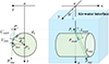 |
Fig. 3 Geometry of the photon colliding with the cylinder target, the left sub-graph is projection of the interaction process. |
where ![Mathematical equation: $ {\overrightarrow{{e}}}_{{i}}=[{U}(y),{U}(z)]$](/articles/jeos/full_html/2026/01/jeos20250088/jeos20250088-eq19.gif) is the unit vector from
is the unit vector from  . For an interaction event, the distance
  ≤ RC (radius of the cross section). The distance
  is expressed as
 (11)
(11)
 in projecting space is converted to three-dimensional space by
 (12)
(12)
and the coordinates of Ptouch then can also be calculated. If Ptouch(x) ![Mathematical equation: $ \in \left[\frac{-{L}_C}{2},\frac{{L}_C}{2}\right]$](/articles/jeos/full_html/2026/01/jeos20250088/jeos20250088-eq26.gif) and the geometric distance of this movement isn’t less than Ltouch, the collision eventually occurs.
and the geometric distance of this movement isn’t less than Ltouch, the collision eventually occurs.
To calculate the direction after collision, the differential tangent plane around  is treated as a Lambertian reflector, so the probability density function of the reflected angle θr can be expressed as
 (13)
(13)
then the propagating direction Ut after collision can be obtained by substituting θr into θ of (7) and the unit direction vector of  into U, where the reflected azimuth angle φr = 2πξrnd. For the upward interaction event, Ut(z) takes a positive value; for the downward interaction event, Ut(z) takes a negative value. The photon’s weight is reduced to Wi = ρWi, and ρ is the surface reflectivity of the target.
2.4 Interaction with the target
Only if the photon’s position Pi is in the volume of detector’s field of view (FOV), the signal contribution can be recorded. The condition of the detection is expressed as [69]![Mathematical equation: $$ \begin{array}{c}\left\{\begin{array}{c}\sqrt{{\left[{{P}}_{{i}}(x)-{{P}}_{\mathbf{FOV}}(x)\right]}^2+{\left[{{P}}_{{i}}(y)-{{P}}_{\mathbf{FOV}}(y)\right]}^2}\enspace \le {R}_1\\ {R}_1=H\cdot \mathrm{tan}\left(\frac{{\theta }_{\mathrm{FOV}}}{2}\right)+{R}_{\mathrm{tele}}+\frac{\left[{{P}}_{{i}}(z)-H\right]\cdot \mathrm{sin}\left(\frac{{\theta }_{\mathrm{FOV}}}{2}\right)}{\sqrt{{n}_w^2-{\mathrm{sin}}^2\left(\frac{{\theta }_{\mathrm{FOV}}}{2}\right)}}\end{array}\right.,\end{array} $$](/articles/jeos/full_html/2026/01/jeos20250088/jeos20250088-eq30.gif) (14)
(14)
where PFOV is the center of the FOV section, and the Rtele is the radius of the telescope. For vertical incidence, PFOV(x) and PFOV(y) are equal to xst and yst. For the oblique incidence, PFOV(x) and PFOV(y) are related to PFOV(z). Figure 4a describes the vertical detection situation when the lidar system is at Pst = [0, 0, 0]. If the photon interacts with the target, Pi is replaced with Ptouch to determine whether the interaction position satisfies the detection condition. The signal contribution of jth photon at position Pi is estimated by [46] (15)
(15)
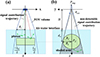 |
Fig. 4 Geometry of photon detection of MCT model. (a) Estimation of water signal (green dotted line) and target reflection signal (red dotted line). (b) The shaded area under the target and non-detectable water signal (gray dotted line). |
where  represents the probability that a photon will be scattered from the current direction to the receiving direction. If the photon interacts with the target,
  is the Lambertian phase function. Otherwise,
  is the phase function of mixed water in equation (8). Ts is the sea surface transmission, Wi is the present weight of the photon. The solid angle of the detector ∆Ω can be calculated by the detector’s image position Pimg = [xst, yst, −nwH + H]. τi is the optical depth from position Pi to lidar position Pst.
However, a special scenario that needs to be considered is when the photon moves underneath the target. As shown in Figure 4, for the vertical detection, the covered extent can be described approximately as![Mathematical equation: $$ \begin{array}{c}\left\{\begin{array}{c}x\in \left[\frac{-{L}_C}{2},\frac{{L}_C}{2}\right]\\ y\in \left[{-R}_2,{R}_2\right]\\ z>H+{d}_w\end{array}\right.,\end{array} $$](/articles/jeos/full_html/2026/01/jeos20250088/jeos20250088-eq35.gif) (16)
(16)
where R2 = dimgtan(θcov/2), dimg = z + H(nw − 1) is distance from the detector’s image position Pimg to the circle center PC, θcov=2sin−1(RC·dimg). When the photon enters this area, the detectable trajectory is blocked by the target, and the photon can no longer make contributions to the signal.
2.5 Interaction with the target
Noise is an influential factor of detection, which mainly includes background signal of solar radiance and detector noise. Nb represents the background signal and is given by [70] (17)
(17)
where Ib is the solar spectral radiance reflected from atmosphere and the water’s surface, A is receiver aperture area, ∆λ is the bandwidth of the detector’s filter, ∆t is the sample time, ηqe is the quantum efficiency of the detector, ηoe is the optical efficiency of the lidar system, λ is the laser wavelength, cv is the speed of light in vacuum, h is the Planck constant. The signal-to-noise ratio of the target signal can be calculated by [70] (18)
(18)
where Nst is the lidar returned photoelectrons with target detection, Nsw is the lidar returned photoelectrons without target (only water detection), Nd is the dark count signal of the detector, and m is the number of the laser shots that need to be integrated.
3 Scanning oceanic lidar system
The airborne linear scanning oceanic lidar system (SOL) for underwater target detection is shown in Figure 5. We chose a 532.1 nm Nd:YAG laser as the light source for strong water penetration. The laser operates reliably over a temperature range of 0–40 °C. Under laboratory conditions at 25 °C, both the output power and pulse energy exhibit stability better than 2%, effectively reducing variations in pulse width and beam quality induced by environmental temperature fluctuations. The photomultiplier tubes (PMT) from the H10720-01 series manufactured by Hamamatsu Photonics are chosen as the detector for good sensitivity and wide dynamic range. The PMT exhibits high cathode radiant sensitivity in the green spectral band and operates reliably over a temperature range of 5–50 °C. Owing to its low dark current, the detector is capable of responding to photon-level signals. The hardware parameters are shown in Table. 1.
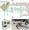 |
Fig. 5 (a) The schematic diagram of SOL system, the laser beam path is in green. Ap is short for aperture stop, CL is short for collimating lens, BF is short for band filter, FL is short for focusing lens, and PBS is short for polarizing beam splitter. (b) SOL is deployed on the UAV. |
Parameters of SOL system.
In the receiving subsystem, a Fresnel lens is selected as the telescope. The telescope has a rear focal length of 60.5 mm and an optical transmittance of up to 96%. The telescope collects the echoes and focuses them onto the rear focal plane. After aperture -stop limitation, the echoes pass through a collimating lens and a narrowband filter to enhance beam collimation and spectral selectivity, suppressing interference from other wavelengths. The conditioned echoes are then separated by a polarizing beam splitter, refocused by focusing lenses, and detected by PMTs, enabling high-sensitivity detection of the return signals.
In the scanning subsystem, a paraxial structure is chosen with the emission subsystem and the receiver subsystem separated at both ends to implement mechanical synchronous scanning. Besides, a reflective photoelectric incremental encoder is equipped to obtain angle information during scanning. It continuously outputs high-resolution TTL pulse signals in A, B, and Z phases. One full rotation corresponds to 163480 pulse signals, yielding a minimum angular resolution of 7.9 arcseconds, which meets the angular accuracy requirements of the UAV-borne lidar system.
4 Model validation
We first simulated water signals and compared them with lidar equation results for model theoretical validation, then simulated the underwater target signals and compared them with the measured profiles to verify the function of the photon’s interaction with target in the model.
4.1 Comparison with lidar equation
The oceanic lidar equation has been broadly applied to validate various lidar signal simulators [47, 49]. The depth-dependent lidar return signal of the lidar equation is [42, 43] (19)
(19)
where zw =z − H is water depth in this study, Ns is the received signal, E is the laser energy for one pulse, O is the overlap factor, ∆tp is the pulse width, Ta is the transmission of atmosphere, v is the frequency of the laser, βπ(z) is the volume scattering coefficient calculated by (6) at the scattering angle of π. Klidar is the lidar attenuation coefficient which is calculated by [43]![Mathematical equation: $$ \begin{array}{c}{K}_{\mathrm{lidar}}\left({z}_w\right)={K}_d\left({z}_w\right)+\left[{c}_{{total}}\left({z}_w\right)-{K}_d\left({z}_w\right)\right]\\ \mathrm{exp}\left[-0.85{c}_{{total}}\left({z}_w\right)D\left({z}_w\right)\right],\end{array} $$](/articles/jeos/full_html/2026/01/jeos20250088/jeos20250088-eq39.gif) (20)
(20)
where ctotal(zw) is the extinction coefficient, Dw(zw) is the lidar spot diameter at different water depth, Kd(zw) is the diffuse attenuation coefficient.
Because of the limitation of lidar equation in dealing with multiple scattering, the water environment has to be as clean as possible to reduce multiple scattering. Referring to Morel’s research, we choose the simulation seawater from the South Pacific anticyclonic gyre (SPG) which is oligotrophic and the “clearest” [57]. Figure 6a shows the chlorophyll concentration profile of SPG water, and the calculated inherent optical properties based on the chlorophyll concentration [43, 57–62].
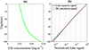 |
Fig. 6 (a) Chlorophyll concentration profile of SPG water, (b) comparison between MC simulation signal and lidar equation signal. |
The relative error used here, which describes how closely the simulated signals match the lidar equation signal, is as follows (21)
(21)
where XS is the simulated value, and XR is the result of lidar equation. We take the mean relative error at 100 m intervals for statistics. We set the number of photons to 107 and take the average results of five simulations for comparison. For simplicity, the MC simulation result and the lidar equation result are normalized based on their respective sea surface signals.
Figure 6b compares the normalized lidar return signals from the lidar equation and the MCT model. A strong agreement between the two results is shown over most depth ranges, indicating the MCT model can accurately reproduce the expected lidar signal attenuation behavior. Slight deviations appear at the deeper water layers, which can be attributed to the cumulative effects of multiple scattering. These effects are inherently captured by the MCT model but simplified in the analytical lidar equation. These deviations can be further characterized through quantitative analysis. The mean relative error is less than 5% within a depth of 50 m and increases to approximately 19.4% at a depth of 100 m. Overall, these results demonstrate that the proposed MCT model achieves high accuracy while providing a more comprehensive and physically realistic description of underwater lidar signal propagation.
4.2 Experiment validation
The measurement experiments of SOL were conducted in the Thousand-Island Lake, Zhejiang province, China. The mean depth of the Thousand-Island Lake is about 34 m, and the maximum depth is more than 100 m. We chose the area near the Gangkou Bridge between two groups of mountains as the experimental area (Fig. 7a). On this occasion, the wind disturbance can be drastically avoided, and the water surface is wide enough. The inherent optical properties of water were measured by Spectral Absorption and Attenuation Sensor ac-s (WET Labs Inc.), and the results are shown in Figure 7b. The green metal barrel was selected as the underwater target. Its length is 0.8 m and its radius is 0.3 m. Its surface has a strong reflection and the reflectivity is about 0.5. As shown in Figure 7c, the ball float and the clump weight were used to fix the metal barrel at a water depth of about 7 m. The lidar SOL was mounted on the UAV DJI Flycart 30. The FPV camera on the UAV can help monitor the surface and assist lidar detection. The direction of flight was perpendicular to the long side of the target (Fig. 7d). Case 1 and case 2 each represent a group of laser beams making up a single linear scanning.
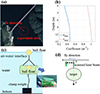 |
Fig. 7 Field experiment of SOL, (a) experimental area in Thousand-Island Lake, (b) the inherent optical properties of experimental water, (c) underwater placement of the target, (d) geometry of the SOL flying over the underwater target. |
The SOL measurements were processed through a series of corrections. In the data pre-processing phase, a low-complexity method based on linear approximation of the leading edge (LLE) was used to extract the water surface precisely, then the slope distances both in the air and water could be calculated as well [71, 72]. Next, according to the angle information of the rotating motor, the slope distances were converted to vertical distances. The one-dimensional signals could be put together as two-dimensional images. Finally, the intensity of the lidar’s output was converted to the number of photoelectrons by calibrating the single-photon response of the detector in the lab.
Figures 8a and 8b show two typical scanning images, and the relevant observed geometries of the UAV that flew over the target are shown in Figure 7d, marked as 1 and 2. Figure 8a was obtained near the top of the target center (case 1), while Figure 8b was obtained from the top edge of the target (case 2). Both of the results had strong signals at a water depth of about 7 m, which revealed the good detection capabilities of SOL. The intensity of the target signals in case 2 was declining and became difficult to distinguish. We also found the signals from the shallow water were so strong that the value was beyond the maximum the data acquisition unit could record. It was the reason that signals from the water surface to about 2 m depth were almost the same.
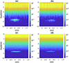 |
Fig. 8 Comparing simulated results with scanned profiles of SOL, (a) and (b) are SOL’s measurements labeled laser beam of 1 and 2 in Figures 6d, 6c and 6d are corresponding simulation results. The color bar represents the number of simulated photoelectrons. |
It is apparent to see the target’s signals at a depth of 7.0 m in the simulated results of Figures 8c and 8d, which is very consistent with the measured results in Figures 8a and 8b. The simulated target’s signals scanned in case 1 are stronger than in case 2. Other than the consistency of the target’s position, the quantity of simulated photoelectrons was consistent with the order of magnitude of measured photons. All of the photoelectron numbers first decreased from 103 at the water surface to about 102.5 at a depth of 3.0 m, then decreased to 101 at 7.0 m. The numbers of photoelectrons from the target were around 102 in case 1 and around 101.5 in case 2. To sum up, the above comparisons demonstrated the correctness of the MCT model.
5 Analysis of the detection capability of SOL
Using the MCT model, the detection capabilities of SOL are further explored. The simulation experiments are carried out under two typical kinds of seawater: Jerlov II and Jerlov 3C [73, 74]. IOPs shown in Figures 9a and 9b are from WOOD (World-wide Ocean Optics Database). The lidar system parameters and the size of the target are the same as in Section 4.2.
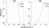 |
Fig. 9 IOPs of Jerlov II (a), Jerlov 3C (b). |
To evaluate the detection differences between two kinds of water, we simulate the signals generated by the target placed at different z-coordinates in case 1, as shown in Figures 10 and 11. The scanning horizontal resolution is 0.4 m. The simulated results show that, when the depth of the target is smaller than 25.0 m in Jerlov II water and 9.0 m in Jerlov 3C water, it is easy to recognize the target. When the z-coordinate of the target is 30.0 m in Jerlov II water and 11.0 m in Jerlov 3C water, the target is barely possible to recognize. Besides, the thickness of the target’s signal, which means its depth range, is greater in Jerlov 3C. This might be relevant to the multiple scattering.
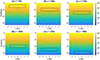 |
Fig. 10 Simulated results of target detection at different depths in Jerlov II water. The color bar represents the number of simulated photoelectrons. |
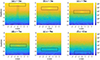 |
Fig. 11 Simulated results of target detection at different depths in Jerlov 3C water. The color bar represents number of simulated photoelectrons. |
Generally speaking, the target recognition of a two-dimensional image is more difficult than that of a single profile. This is because in a two-dimensional image, there must be continuous target features (at least two continuous profiles) to be convincing. As shown in Figures 10 and 11, the strongest target signals exist near the center of it (x = 0), and decrease with horizontal distance from the center. Based on the results of Figures 10 and 11, we simulate the detection capability of a single profile of multiple z-coordinates of the target in case 1. We use Nst−Nsw to acquire the signals that are only reflected by the target. The feature peaks of Nst−Nsw signals with different depths are extracted and plotted as Figure 12a. The signal-to-noise ratios of these feature peaks are calculated and shown as Figure 12b. It can be seen that the photoelectron numbers in both water environments go down exponentially with depth, and in Jerlov 3C water, they decrease much faster because of the bigger attenuation coefficients. The same trend appears in the distribution of target signal SNR with respect to depth, as shown in Figure 12b.
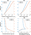 |
Fig. 12 Analysis of simulation results for target detection at different depths in Jerlov II water and Jerlov 3C water, (a) simulated numbers of photoelectrons, (b) SNR of target signals, (c) extended detection range of different depths, (d) horizontal resolution of the scanning in x-axis of different depths. |
It is widely known that SNR can be improved by integrating several profiles. To improve the SNR of Nst−Nsw, the horizontal sampling interval should be reduced so that more laser shots are able to encounter the target. We have already discovered that the horizontal detectable length range of target is beyond its actual length [xϵ (−0.4 m, 0.4 m)] (Figs. 10 and 11). Therefore, after counting the number of photoelectrons with horizontal distribution at the same depth of target, the definition of extended detection range is made as the x-range when the photoelectron numbers with target reduce to half of that at the center top (x = 0). The statistical results of the extended detection range are displayed in Figure 12c. Assume the SNR does not change within this range, and set SNR = 3 as the standard. Then the relationships between max detectable depth and horizontal scanning resolution of Jerlov II and Jerlov 3C water are shown in Figure 12d by interpolating at the depth resolution of 0.1 m. Only one single profile is needed when the target depth is shallower than 25.0 m in Jerlov II water and 9.2 m in Jerlov 3C water, so the max point resolutions are equal to the extended detection ranges. It should be noted that the phenomenon of photoelectron numbers of the target dropping to half does not mean the target cannot be recognized. Recognition still depends on its true value and SNR (Fig. 10a). As the depths of target add up, more and more profiles have to be integrated, so the point resolutions are equal to the corresponding extended detection range divided by the number of integrated profiles. If the SNR reduces to a very small value, like lower than 1, it will be better to level up the number of integrated four times as calculated by equation (18).
The preceding analysis reveals that, to achieve a certain target SNR, deeper targets require the integration of more lidar profiles to enhance signal quality. This requires an increase in horizontal sampling density to ensure that more laser beams effectively interact with the target. While this approach improves the detectability of deep targets, it simultaneously reduces the area that can be covered within a given time, thereby decreasing the overall detection efficiency. This compromise carries important scientific implications for the design and operation of oceanic scanning lidar systems for target detection. Firstly, it quantitatively links detection depth to the required lidar signal profiles integration, and offers a theoretical basis for estimating detection costs at varying depths. Secondly, it highlights the inherent constraint between detection depth and operational efficiency and emphasizes the balance of spatial resolution, scanning speed, and signal quality in system configuration. This understanding provides valuable guidance for making acquisition strategies to different targets and water environments.
6 Conclusion
Oceanic lidar is significant for detecting deeper water. In this study, we proposed a semi-analytic MC model of underwater target detection (MCT) and developed an airborne linear scanning oceanic lidar system (SOL) for model validation. The comparison is made between lidar equation signals and MC simulated signals to validate the correctness of our model. It turns out the mean relative error is less than 5% within a depth of 50 m and is about 19.4% within a depth of 100 m. By comparing the simulated two-dimensional scanning signals with SOL’s field target measurements, the measured results show the consistency of the target’s position and the order of magnitude of photoelectrons. Then a series of simulations in Jerlov II water and Jerlov 3C water are made to study the detection capabilities of SOL. It turns out that, set SNR = 3 as the detection standard, the maximum target detection depths are 25.0 m in Jerlov II water and 9.2 m for a single profile. The definition of extended detection range is made, and how the maximum horizontal scanning resolution varies with depth is studied as well. Their relationships are conducive to balancing detection capabilities and scanning efficiency, providing a good reference for practical detection scenes. By exploring a range of representative simulation conditions, including different water optical types, target depths, and scanning parameters, the proposed MCT model is shown to be robust and effective. In addition to the cases presented in this work, the model framework is readily extensible to other scenarios involving variations in lidar system parameters and target-related properties, such as target size, shape and reflectivity.
There are also limitations to the MCT, such as the floating ball interference. In practical field measurements, floating balls can generate strong reflective signals at the sea surface, introducing additional non-target returns and locally increasing background levels. Such surface-related reflections may reduce the contrast of target echoes under certain conditions. In addition, other detector-related noise such as the after pulse, manifests primarily as weak delayed components in the received waveforms, which may cause a slight overestimation of deep-water signals. These effects will be further investigated in future studies. Furthermore, a more comprehensive parametric study about diverse water optical properties and lidar system parameters will be essential to construct generalized models, which can improve the transferability and applicability of the simulated findings in the broader practical scenarios.
Funding
This work is supported by the National Key Research and Development Program of China (Grant No. 2022YFB3901701).
Conflicts of interest
The authors declare that there are no financial interests, commercial affiliations, or other potential conflicts of interest that could have influenced the objectivity of this research or the writing of this paper.
Data availability statement
The data underlying the results presented in this paper is not publicly available at this time but may be provided upon reasonable request to the corresponding author.
Author contribution statement
All authors have reviewed, discussed, and agreed to their individual contributions. The specific situation is as follows: Methodology, Xinke Hao and Yan He; Data Curation, Xinke Hao, Yingjie Ruan and Hui Qi; Writing – Original Draft Preparation, Xinke Hao and Huixin He; Writing – Review and Editing, Huixin He and Yan He; Supervision, Deliang Lv and Guangxiu Xu; Project Administration, Yan He and Junwu Tang; Funding Acquisition, Yan He.
References
- Wölfl AC et al., Seafloor mapping – The challenge of a truly global ocean bathymetry, Front. Mar. Sci. 6, 283 (2019). https://doi.org/10.3389/fmars.2019.00283. [Google Scholar]
- Leifer I et al., State-of-the-art satellite and airborne marine oil spill remote sensing: Application to the BP deepwater horizon oil spill, Remote Sens. Environ. 124, 185–209 (2012). https://doi.org/10.1016/j.rse.2012.03.024. [Google Scholar]
- Sathyendranath S, et al., Ocean-colour products for climate-change studies: What are their ideal characteristics?, Remote Sens. Environ. 203, 125–138 (2017). https://doi.org/10.1016/j.rse.2017.04.017. [Google Scholar]
- Li Z et al., Exploring modern bathymetry: A comprehensive review of data acquisition devices, model accuracy, and interpolation techniques for enhanced underwater mapping, Front. Mar. Sci. 10, 1178845 (2023). https://doi.org/10.3389/fmars.2023.1178845. [Google Scholar]
- Matte G et al., Implementation of the split-beam function to Mills cross multibeam echo sounder for target strength measurements, ICES J. Mar. Sci. 81(7), 1424–1433 (2024). https://doi.org/10.1093/icesjms/fsae032. [Google Scholar]
- Jamet C et al., Going beyond standard ocean color observations: Lidar and polarimetry, Front. Mar. Sci. 6, 251 (2019). https://doi.org/10.3389/fmars.2019.00251. [Google Scholar]
- Ashphaq M et al., Review of near-shore satellite derived bathymetry: Classification and account of five decades of coastal bathymetry research, J. Ocean Eng. Sci. 6(4), 340–359 (2021). https://doi.org/10.1016/j.joes.2021.02.006. [Google Scholar]
- Chowdhury E et al., Use of bathymetric and LiDAR data in generating digital elevation model over the Lower Athabasca River Watershed in Alberta, Canada, Water 9, 19 (2017). https://doi.org/10.3390/w9010019. [Google Scholar]
- Chen Y et al., Simulation and design of an underwater lidar system using non-coaxial optics and multiple detection channels, Remote Sens. 15, 3618 (2023). https://doi.org/10.3390/rs15143618. [Google Scholar]
- Eren F et al., Bottom characterization by using airborne lidar bathymetry (ALB) waveform features obtained from bottom return residual analysis, Remote Sens. Environ. 206, 260–274 (2018). https://doi.org/10.1016/j.rse.2017.12.035. [Google Scholar]
- Hoge FE et al., Water depth measurement using an airborne pulsed neon laser system, Appl. Opt. 19(6), 871–883 (1980). https://doi.org/10.1364/AO.19.000871. [Google Scholar]
- Irish JL et al., Airborne lidar bathymetry: The SHOALS system, Bot. Int. Navig. Assoc. 43–53 (2000). [Google Scholar]
- LaRocque PE et al., Design description and field testing of the SHOALS-1000T airborne bathymeter, in Proc. SPIE 5412, Laser Radar Technology and Applications IX (2004). https://doi.org/10.1117/12.564924. [Google Scholar]
- Mandlburger G et al., A decade of progress in topo-bathymetric laser scanning exemplified by the Pielach River dataset, ISPRS Ann. Photogramm. Remote Sens. Spatial Inf. Sci. X-1/W1-2023, 1123–1130 (2023). https://doi.org/10.5194/isprs-annals-X-1-W1-2023-1123-2023. [Google Scholar]
- Steinbacher F et al., High resolution, topobathymetric LiDAR coastal zone characterization in Denmark, HYDRO 2016, 2016. [Google Scholar]
- Wilson N et al., Mapping seafloor relative reflectance and assessing coral reef morphology with EAARL-B topobathymetric lidar waveforms, Estuaries Coasts 45, 923–937 (2022). https://doi.org/10.1007/s12237-019-00652-9. [Google Scholar]
- Feygels VI et al., CZMIL (Coastal Zone Mapping and Imaging Lidar): From first flights to first mission through system validation, in Proc. Ocean Sensing and Monitoring V, 8724 (2013). https://doi.org/10.1117/12.2017935. [Google Scholar]
- Moore TS et al., Vertical distributions of blooming cyanobacteria populations in a freshwater lake from lidar observations, Remote Sens. Environ. 225, 347–367 (2019). https://doi.org/10.1016/j.rse.2019.02.025. [Google Scholar]
- Churnside JH et al., Airborne remote sensing of a biological hot spot in the southeastern Bering Sea, Remote Sens. 3(3), 621–637 (2011). https://doi.org/10.3390/rs3030621. [Google Scholar]
- Chen P et al., Vertical distribution of subsurface phytoplankton layer in South China Sea using airborne lidar, Remote Sens. Environ. 263, 112567 (2021). https://doi.org/10.1016/j.rse.2021.112567. [Google Scholar]
- Liu H et al., Subsurface plankton layers observed from airborne lidar in Sanya Bay, South China Sea, Opt. Express 26, 29134–29147 (2018). https://doi.org/10.1364/OE.26.029134. [Google Scholar]
- Schulien JA et al., Vertically-resolved phytoplankton carbon and net primary production from a high spectral resolution lidar, Opt. Express 25(12), 13577–13587 (2017). https://doi.org/10.1364/OE.25.013577. [Google Scholar]
- Chen W et al., Review of airborne oceanic lidar remote sensing, Intell. Mar. Technol. Syst. 1(1), 10 (2023). https://doi.org/10.1007/s44295-023-00007-y. [Google Scholar]
- Churnside JH et al., Airborne lidar for fisheries applications, Opt. Eng. 40(3), 406–414 (2001). https://doi.org/10.1117/1.1348000. [Google Scholar]
- Roddewig MR et al., Dual-polarization airborne lidar for freshwater fisheries management and research, Opt. Eng. 56(3), 031221 (2017). https://doi.org/10.1117/1.OE.56.3.031221. [Google Scholar]
- Scofeld TP et al., Applying Gaussian mixture models to detect fish from airborne lidar measurements, in Proc. IEEE Res. Appl. Photon. Def. Conf. (RAPID), Miramar Beach (2021). https://doi.org/10.1109/RAPID51799.2021.9521457. [Google Scholar]
- Churnside JH et al., Surveying the distribution and abundance of flying fishes and other epipelagic in the northern Gulf of Mexico using airborne lidar, Bull. Mar. Sci. 93(2), 591–609 (2016). https://doi.org/10.5343/bms.2016.1039. [Google Scholar]
- Churnside JH et al., Ocean backscatter profiling using high-spectral-resolution lidar and a perturbation retrieval, Remote Sens. 10(12), 2003 (2018). https://doi.org/10.3390/rs10122003. [Google Scholar]
- Liu Q et al., Shipborne variable-FOV, dual-wavelength, polarized ocean lidar: design and measurements in the Western Pacific, Opt. Express 30, 8927 (2022). https://doi.org/10.1364/OE.449554. [Google Scholar]
- Li K et al., A dual-wavelength ocean lidar for vertical profiling of oceanic backscatter and attenuation, Remote Sens. 12, 2844 (2020). https://doi.org/10.3390/rs12172844. [Google Scholar]
- Chen P et al., LiDAR remote sensing for vertical distribution of seawater optical properties and chlorophyll-a from the East China Sea to the South China Sea, IEEE Trans. Geosci. Remote Sens. 60, 1–21 (2022). https://doi.org/10.1109/TGRS.2022.3174230. [CrossRef] [Google Scholar]
- Lee JH et al., Oceanographic lidar profiles compared with estimates from in situ optical measurements, Appl. Opt. 52(4), 786–794 (2013). https://doi.org/10.1364/AO.52.000786. [Google Scholar]
- Zhang L et al., An experimental study on monitoring wave profiles with lidar, Ocean Eng. 285, 115436 (2023). https://doi.org/10.1016/j.oceaneng.2023.115436. [Google Scholar]
- Wang D et al., An experimental study on measuring breaking-wave bubbles with lidar remote sensing, Remote Sens. 14(7), 12 (2022). https://doi.org/10.3390/rs14071680. [Google Scholar]
- Churnside JH et al., Airborne lidar detection and characterization of internal waves in a shallow fjord, J. Appl. Remote Sens. 6, 063611 (2012). https://doi.org/10.1117/1.JRS.6.063611. [Google Scholar]
- Dolin LS et al., Algorithms for determining the spectral-energy characteristics of a random field of internal waves from fluctuations of lidar echo signals, Appl. Opt. 59(10), C78–C86 (2020). https://doi.org/10.1364/AO.381675. [Google Scholar]
- Maccarone A et al., Three-dimensional imaging of stationary and moving targets in turbid underwater environments using a single-photon detector array, Opt. Express 27(20), 28437–28456 (2019). https://doi.org/10.1364/OE.27.028437. [Google Scholar]
- Maccarone A et al., Submerged single-photon lidar imaging sensor used for real-time 3D scene reconstruction in scattering underwater environments, Opt. Express 31(10), 19(2023). https://doi.org/10.1364/OE.487129. [Google Scholar]
- Shangguan M et al., Compact underwater single-photon imaging lidar, Opt. Lett. 50(6), 1957–1960 (2025). https://doi.org/10.1364/OL.557195. [Google Scholar]
- Yang E et al., SHOALS object detection, Int. Hydrogr. Rev. 24–36 (2010). [Google Scholar]
- Wang D et al., Evaluation of a new lightweight UAV-borne topo-bathymetric lidar for shallow water bathymetry and object detection, Sensors 22(4), 1379 (2022). https://doi.org/10.3390/s22041379. [Google Scholar]
- Zhang Z et al., SOLS: An open-source spaceborne oceanic lidar simulator, Remote Sens. 14, 1849 (2022). https://doi.org/10.3390/rs14081849. [Google Scholar]
- Churnside JH, Review of profiling oceanographic lidar, Opt. Eng. 53, 051405 (2013). https://doi.org/10.1117/1.OE.53.5.051405. [Google Scholar]
- Zhou Y et al., Validation of the analytical model of oceanic lidar returns: Comparisons with Monte Carlo simulations and experimental results, Remote Sens. 11, 1870 (2019). https://doi.org/10.3390/rs11161870. [Google Scholar]
- Liao Y et al., GPU-accelerated Monte Carlo simulation for a single-photon underwater lidar, Remote Sens. 15, 5245 (2023). https://doi.org/10.3390/rs15215245. [Google Scholar]
- Poole LR et al., Semianalytic Monte Carlo radiative transfer model for oceanographic lidar systems, Appl. Opt. 20, 3653–3663 (1981). https://doi.org/10.1364/AO.20.003653. [Google Scholar]
- Liu Q et al., A semianalytic Monte Carlo simulator for spaceborne oceanic lidar: Framework and preliminary results, Remote Sens. 12, 2820 (2020). https://doi.org/10.3390/rs12172820. [Google Scholar]
- Stegmann PG et al., Study of the effects of phytoplankton morphology and vertical profile on lidar attenuated backscatter and depolarization ratio, J. Quant. Spectrosc. Radiat. Transf. 225, 1–15 (2019). https://doi.org/10.1016/j.jqsrt.2018.12.009. [Google Scholar]
- He H et al., Validation of the polarized Monte Carlo model of shipborne oceanic lidar returns, Opt. Express 31, 43250 (2023). https://doi.org/10.1364/OE.511445. [Google Scholar]
- Cui X et al., Influence of wind-roughed sea surface on detection performance of spaceborne oceanic lidar, J. Quant. Spectrosc. Radiat. Transf. 297, 108481 (2023). https://doi.org/10.1016/j.jqsrt.2022.108481. [Google Scholar]
- Chen P et al., OLE: A novel oceanic lidar emulator, IEEE Trans. Geosci. Remote Sens. 59, 9730–9744 (2021). https://doi.org/10.1109/TGRS.2020.3035381. [Google Scholar]
- Chen P et al., Semi-analytic Monte Carlo model for oceanographic lidar systems: Lookup table method used for randomly choosing scattering angles, Appl. Sci. 9, 48 (2018). https://doi.org/10.3390/app9010048. [Google Scholar]
- Wang CK et al., A Monte Carlo study of the seagrass-induced depth bias in bathymetric lidar, Opt. Express 19, 7230 (2011). https://doi.org/10.1364/OE.19.007230. [Google Scholar]
- Li J et al., Range difference between shallow and deep channels of airborne bathymetry lidar with segmented field-of-view receivers, IEEE Trans. Geosci. Remote Sens. 60, 1–16 (2022). https://doi.org/10.1109/TGRS.2022.3172351. [CrossRef] [Google Scholar]
- Guo S et al., Monte Carlo simulation with experimental research about underwater transmission and imaging of laser, Appl. Sci. 12(18), 8959 (2022). https://doi.org/10.3390/app12188959. [Google Scholar]
- Huang Y et al., Semi-analytical Monte Carlo simulation of underwater target echoes from a small UAV-based oceanic lidar, Opt. Commun. 574, 131157(2025). https://doi.org/10.1016/j.optcom.2024.131157. [Google Scholar]
- Morel A et al., Optical properties of the ‘clearest’ natural waters, Limnol. Oceanogr. 52, 217–229 (2007). https://doi.org/10.4319/lo.2007.52.1.0217. [NASA ADS] [CrossRef] [Google Scholar]
- Morel A et al., Bio-optical properties of oceanic waters: A reappraisal, J. Geophys. Res. Oceans 106, 7163–7180 (2001). https://doi.org/10.1029/2000JC000319. [Google Scholar]
- Bricaud A et al., Variations of light absorption by suspended particles with chlorophyll a concentration in oceanic (case 1) waters: Analysis and implications for bio-optical models, J. Geophys. Res. Oceans 103, 31033–31044 (1998). https://doi.org/10.1029/98JC02712. [Google Scholar]
- Bricaud A, et al., Absorption by dissolved organic matter of the sea (yellow substance) in the UV and visible domains, Limnol. Oceanogr. 26, 43–53(1981). https://doi.org/10.4319/lo.1981.26.1.0043. [CrossRef] [Google Scholar]
- Pope RM et al., Absorption spectrum (380–700 nm) of pure water II: Integrating cavity measurements, Appl. Opt. 36, 8710 (1997). https://doi.org/10.1364/AO.36.008710. [NASA ADS] [CrossRef] [Google Scholar]
- Nelson NB et al., The global distribution and dynamics of chromophoric dissolved organic matter, Annu. Rev. Mar. Sci. 5, 447–476 (2013). https://doi.org/10.1146/annurev-marine-120710-100751. [NASA ADS] [CrossRef] [Google Scholar]
- Levy U et al., Mathematics of vectorial Gaussian beams, Adv. Opt. Photonics 11, 828 (2019). https://doi.org/10.1364/AOP.11.000828. [Google Scholar]
- Cox C, Munk W, Measurement of the roughness of the sea surface from photographs of the sun’s glitter, J. Opt. Soc. Am. 44(11), 838–50 (1954). https://doi.org/10.1364/JOSA.44.000838. [NASA ADS] [CrossRef] [Google Scholar]
- Leathers RA et al., Monte Carlo radiative transfer simulations for ocean optics: A practical guide, (2004). https://doi.org/10.21236/ADA426624. [Google Scholar]
- Petzold TJ, Volume scattering functions for selected ocean waters (Scripps Inst. Oceanogr., San Diego, CA, USA, 1972). https://doi.org/10.21236/AD0753474. [Google Scholar]
- Mobley CD et al., Phase function effects on oceanic light fields, Appl. Opt. 41, 1035 (2002). https://doi.org/10.1364/AO.41.001035. [NASA ADS] [CrossRef] [Google Scholar]
- Mobley CD et al., Comparison of numerical models for computing underwater light fields, Appl. Opt. 32, 7484 (1993). https://doi.org/10.1364/AO.32.007484. [NASA ADS] [CrossRef] [Google Scholar]
- Yin T et al., Simulation of satellite, airborne and terrestrial lidar with DART (II): ALS and TLS multi-pulse acquisitions, photon counting, and solar noise, Remote Sens. Environ. 184, 454–468 (2016). https://doi.org/10.1016/j.rse.2016.07.009. [Google Scholar]
- Liu Z et al., Simulations of the observation of clouds and aerosols with the Experimental Lidar in Space Equipment system, Appl. Opt. 39, 3120 (2000). https://doi.org/10.1364/AO.39.003120. [Google Scholar]
- Pan Z et al., Performance assessment of high resolution airborne full waveform lidar for shallow river bathymetry, Remote Sens. 7, 5133–5159 (2015). https://doi.org/10.3390/rs70505133. [Google Scholar]
- Tao B, et al., Precise detection of water surface through the analysis of a single green waveform from bathymetry lidar, Opt. Express 30, 40820 (2022). https://doi.org/10.1364/OE.468404. [Google Scholar]
- Smart JH, World-wide Ocean Optics Database (WOOD) 1900–2011 (NCEI Accession 0092528), NOAA National Centers for Environmental Information, Dataset (2012). https://www.ncei.noaa.gov/archive/accession/0092528. [Google Scholar]
- Sauzède R et al., A neural network-based method for merging ocean color and Argo data to extend surface bio-optical properties to depth: Retrieval of the particulate backscattering coefficient, J. Geophys. Res. Oceans 121, 2552–2571 (2016). https://doi.org/10.1002/2015JC011408. [Google Scholar]
All Tables
All Figures
|
Fig. 1 Flow chart of MCT simulation model. |
| In the text | |
|
Fig. 2 (a) Global coordinate system of the simulation model, and (b) sampling the point from the Gaussian spot. |
| In the text | |
|
Fig. 3 Geometry of the photon colliding with the cylinder target, the left sub-graph is projection of the interaction process. |
| In the text | |
|
Fig. 4 Geometry of photon detection of MCT model. (a) Estimation of water signal (green dotted line) and target reflection signal (red dotted line). (b) The shaded area under the target and non-detectable water signal (gray dotted line). |
| In the text | |
|
Fig. 5 (a) The schematic diagram of SOL system, the laser beam path is in green. Ap is short for aperture stop, CL is short for collimating lens, BF is short for band filter, FL is short for focusing lens, and PBS is short for polarizing beam splitter. (b) SOL is deployed on the UAV. |
| In the text | |
|
Fig. 6 (a) Chlorophyll concentration profile of SPG water, (b) comparison between MC simulation signal and lidar equation signal. |
| In the text | |
|
Fig. 7 Field experiment of SOL, (a) experimental area in Thousand-Island Lake, (b) the inherent optical properties of experimental water, (c) underwater placement of the target, (d) geometry of the SOL flying over the underwater target. |
| In the text | |
|
Fig. 8 Comparing simulated results with scanned profiles of SOL, (a) and (b) are SOL’s measurements labeled laser beam of 1 and 2 in Figures 6d, 6c and 6d are corresponding simulation results. The color bar represents the number of simulated photoelectrons. |
| In the text | |
|
Fig. 9 IOPs of Jerlov II (a), Jerlov 3C (b). |
| In the text | |
|
Fig. 10 Simulated results of target detection at different depths in Jerlov II water. The color bar represents the number of simulated photoelectrons. |
| In the text | |
|
Fig. 11 Simulated results of target detection at different depths in Jerlov 3C water. The color bar represents number of simulated photoelectrons. |
| In the text | |
|
Fig. 12 Analysis of simulation results for target detection at different depths in Jerlov II water and Jerlov 3C water, (a) simulated numbers of photoelectrons, (b) SNR of target signals, (c) extended detection range of different depths, (d) horizontal resolution of the scanning in x-axis of different depths. |
| In the text | |
Current usage metrics show cumulative count of Article Views (full-text article views including HTML views, PDF and ePub downloads, according to the available data) and Abstracts Views on Vision4Press platform.
Data correspond to usage on the plateform after 2015. The current usage metrics is available 48-96 hours after online publication and is updated daily on week days.
Initial download of the metrics may take a while.