| Issue |
J. Eur. Opt. Society-Rapid Publ.
Volume 21, Number 1, 2025
EOSAM 2024
|
|
|---|---|---|
| Article Number | 19 | |
| Number of page(s) | 12 | |
| DOI | https://doi.org/10.1051/jeos/2025016 | |
| Published online | 29 April 2025 | |
Research Article
Investigation of the positioning accuracy of the Cat’s Eye as a reference position in asphere-measuring interferometry
Physikalisch-Technische Bundesanstalt (PTB), Bundesallee 100, 38116 Braunschweig, Germany
* Corresponding author: This email address is being protected from spambots. You need JavaScript enabled to view it.
Received:
29
January
2025
Accepted:
31
March
2025
Abstract
The increasing interest of the optics manufacturing industry in apshere and freeform optics leads to a high demand in accurate form measurement of such surfaces. The tilted-wave interferometer offers a fast and flexible solution to the needs. However, similar to other interferometric methods, ambiguities between specimen misalignment and certain form errors exist. To ensure the accuracy of the form measurement, the accuracy of the specimen positioning is crucial. This work presents a multi-step specimen positioning procedure that uses the Cat’s Eye reference position as a fixed reference position. Different alignment criteria are evaluated by simulation and implemented into an alignment algorithm for specimen alignment into the Cat’s Eye position. The procedure, investigated with multiple test specimens, shows a good short-term repeatability with a standard deviation below 30 nm. The use of this specimen alignment procedure will significantly reduce surface form measurement errors associated with axial misalignment and improve the overall measurement accuracy of the tilted-wave interferometer.
Key words: Interferometric form measurement / Asphere metrology / Surface positioning
© The Author(s), published by EDP Sciences, 2025
 This is an Open Access article distributed under the terms of the Creative Commons Attribution License (https://creativecommons.org/licenses/by/4.0), which permits unrestricted use, distribution, and reproduction in any medium, provided the original work is properly cited.
1 Introduction
Modern optical technology utilizes aspherical and freeform optics more and more for their inherent capability of correcting optical aberrations, which gives these optical elements an advantage over classic spherical optics [1, 2]. This has led to more compact, yet high-quality, optical systems both in professional and consumer devices. The advancements in usage and design of optical aspheres and freeforms have led to an increasing demand in measurement technology for these surfaces, since highly accurate manufacturing is fundamentally limited by the accuracy with which the surfaces to be manufactured can be characterized. Measurement methods for such surfaces can be divided into point-based and area-based approaches. Point-based approaches use either an optical [3] or a tactile probe [4] to scan the surface under test. These methods are highly adaptable in regards to the surface form that can be measured. However, the serial nature of the approach leads to a trade-off between measurement time and lateral resolution. Area-based methods on the other hand can achieve both short measurement times and high lateral resolution due to their parallel measurement approach. They are usually based on interferometry [5] or deflectometry [6] and have typically more limitations in regards of the surface form that can be measured. In contrast to spherical optics, which can be measured easily by interferometric null-test, the measurement of aspherical or freeform optics is much more challenging [7]. Here, an interferometric null-test would require a custom-made reference for every desired specimen, which is often done utilizing a computer-generated hologram (CGH) that has to be calculated and fabricated with lithographic methods. Measurement with CGHs requires meticulous effort in specimen alignment or else can lead to large measurement errors. For small series or individual specimens, this approach is too costly and time-consuming to be feasible. Therefore, for this use-case interest has shifted away from interferometric null-test to non-null-test measurement approaches such as subaperture stitching interferometry [8], axial scanning interferometry [9], or sub-Nyquist interferometry [10].
A very promising optical method for such measurements is tilted-wave interferometry [11–13]. A tilted-wave interferometer (TWI) combines a special interferometer setup with model-based data evaluation methods. The setup is a modified Twyman-Green interferometer, in which a microlens array is added to the objective arm such that the specimen is illuminated by differently tilted wavefronts instead of a single wavefront. In contrast to the null-test scenario of spherical form measurement, a common path between incident and reflected wavefront is not necessary and the imaged interference patches just represent resolvable interference fringes without direct information about the form deviation of the specimen. Instead, to reconstruct the specimen from the interferograms, an inverse problem has to be solved. For this purpose, a digital twin of the measurement setup, including the interferometer and a virtual specimen is needed to simulate the interferograms for the design of the specimen. With this, optical path length differences are simulated by ray tracing and ray aiming [14]. The simulated data are then compared to the data that are extracted from the measured interferograms [15, 16]. The form of the surface under test is then reconstructed by solving an inverse problem minimizing the difference between the simulated and measured data. Since a model of the setup is used, the model has to be adapted to the real system. This is done in a special calibration procedure that utilizes well-known reference specimens in a large number of measurement positions. For a detailed description of the digital twin modeling, the model correction, and the reconstruction process that is utilized at the Physikalisch-Technische Bundesanstalt (PTB), please refere to [17].
However, as with interferometric form measurement in general, TWI measurements also suffer from ambiguities between surface form errors and misalignment of the specimen [18]. For TWI measurements, the form measurement accuracy is especially affected by misalignment along the optical axis of the interferometer [19]. In order to resolve this ambiguity, additional external positioning information can be used to better align the surface positioning between the experiment and the modeling. Previous simulation studies have shown that a single absolute length information with an accuracy of 100 nm or better could reduce the surface form measurement error contribution of the alignment down to a few nanometers root-mean-square (RMS) [19].
To achieve this, accurate and repeatable specimen positioning methods, especially for positioning along the optical axis (z), are required. Therefore, at PTB, a multi step approach for the specimen positioning in a TWI is developed: First, the specimen is aligned into the so-called Cat’s Eye position, which is a common reference position in interferometric form measurement [20]. The Cat’s Eye position is defined as the position in which the focus of the interferometer’s objective coincides with the specimen’s surface. Because of that, all light gets reflected in a single spot, making the Cat’s Eye theoretically independent of the measurement surface form. Therefore, the Cat’s Eye only depends on the optical system of the interferometer, which leads to a well-defined criterion for surface positioning. From there, the specimen is moved into the measurement position while the positioning stage is tracked by a distance measuring interferometer (DMI). This ties the positioning accuracy of the axial positioning in measurement position effectively to the positioning accuracy of the Cat’s Eye position. In a next step, the measurement position is used to align the surface laterally (x and y) as well as its tilt (α and β, depending on the degrees of freedom of the surface under test). In measurement position, the sensitivity coefficients between the optical path length difference changes with regard to positioning can be used. This step will be investigated in future work in more detail. Since a lateral repositioning also has influence on the axial position, after the positioning optimization in measurement position, the specimen is moved back to the Cat’s Eye reference position and the axial positioning procedure is repeated without changing the lateral position. Finally, the specimen is moved to the measurement position while the positioning stage is tracked by the DMI. The two important positions are the Cat’s Eye position and the measurement position illustrated in Figure 1.
 |
Figure 1 Specimen positioning within the TWI. (a) Specimen positioned in the Cat’s Eye reference position. (b) Specimen moved to the measurement position, tracked by a distance-measuring interferometer (DMI). |
In this work, we present a method of adjusting the specimen into the Cat’s Eye position in the TWI and show its repeatability. In Section 2 the measurement system and the utilized methods are described. In Section 3, the results of the repeated measurements are presented and discussed. Finally, Section 4 sets the results of our approach into the context of the TWI form reconstruction and discusses future challenges.
2 Method
2.1 Tilted-wave interferometer setup
Both for analyzing the interferograms of specimens in or near the Cat’s Eye reference position and for generating test data for the positioning algorithm, virtual interference images are generated utilizing a digital twin of the TWI at PTB. The digital twin consists of a ray tracing simulation that simulates every optical surface in the instrument. It is built in MATLAB and utilizes the in-house developed ray tracing and ray aiming library SimOptDevive [14]. For further details on the implementation of the TWI simulation and the TWI measurement procedure, please refer to [17]. The general optical setup of the TWI, and therefore also of the digital twin, is depicted in Figure 2a.
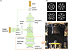 |
Figure 2 (a) Optical setup of the TWI. (b) Example of four camera images with the sub-interferograms of an aspherical specimen created by the four mask positions of the microlens array. (c) Photo of the specimen stage of the TWI showing a specimen and the TWI objective. |
The optical setup of the TWI utilizes a Nd:YAG laser with a wavelength of λ = 532.3 nm as illumination light source. The light is divided by a beamsplitter into a primary object wavefront and a reference wavefront. The reference wavefront is guided into an optical fiber, while the primary object wavefront is widened, collimated, and cast onto a microlens array [21]. The microlens array then generates multiple secondary object wavefronts that are then collimated and projected by an objective onto the specimen. The different locations of the microlenses in the plane of the microlens array are transformed into differently tilted wavefronts at the specimen. The wavefronts are then reflected at the specimen and then travel back through the objective and collimator and are projected onto the image detector. The reflected wavefronts interfere with the reference wavefront behind the beamsplitter and a rectangular beam stop in the Fourier plane of the imaging optics acts as a spatial frequency filter and therefore avoids subsampling effects on the camera. Depending on the local slope of the surface under test different parts of the differently tilted and reflected wavefronts arrive at the camera leading to several sub-interferograms (patches). In order to avoid overlapping patches and interference of light from neighboring microlenses, a beam stop grid selectively blocks every second row and column of the microlenses, leading with 4 different grid positions to 4 different camera images (Fig. 2(b)). A small section of the real setup, including the specimen stage, a specimen and the TWI objective is shown in Figure 2c. For further information on the TWI setup and the image formation please refer to [11, 13, 17, 19, 21–24].
2.2 Simulation of specimen position influence on interferograms
For evaluating interferograms in or near the Cat’s Eye reference position, a virtual specimen of an asphere [25] is placed in the desired position in the model and the interferograms are simulated. For the specimen positioning in the Cat’s Eye position only the central, on-axis microlens of the microlens array is required. In the physical TWI, this configuration can be selected by an iris diaphragm in front of the beam stop grid. Therefore, only rays from the central microlens are simulated. The illumination light gets reflected back by the surface under test, travels through the optical system, is deflected at the beam splitter between the microlens array and the collimator and is cast on the detector by the secondary imaging system. A surface in the Cat’s Eye position leads to the reflected light having a focal point in the plane of the rectangular beam stop (compare Fig. 2). However, when the surface shifts away from the Cat’s Eye, the reflection is no longer in a singular point and the focal point moves out of the plane of the beam stop. At a certain distance, the beam stop begins to clip the edges of the backreflected light. This leads to an image of the beam stop being visible on the image detector and causes the rectangular shape of the interferograms shown in Figure 3. When the surface is additionally moved in lateral direction, the movement of the focal point causes a lateral shift of the beam stop’s image. In Figure 3, simulated interferograms of different specimen positions around the Cat’s Eye reference position are shown.
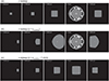 |
Figure 3 Interferograms for a specimen (asphere) positioned in different positions around the Cat’s Eye reference position. (a) Sweep along the optical axis (z). (b) Sweep perpendicular to the optical axis (lateral sweep in x) in the plane of the Cat’s Eye position. (c) Sweep perpendicular to the optical axis in a plane 1 mm away from the Cat’s Eye position. |
The interferograms of a specimen sweep along the optical axis (z-axis) are shown in Figure 3a. In the Cat’s Eye position (z = 0 μm), the interferogram is not limited by the beam stop and has a circular shape. The further away the specimen’s apex is from this position, the more the interferogram is limited by the beam stop aperture, leading to a rectangular shape that gets smaller with larger distances to the Cat’s Eye position. When the specimen is moved perpendicular to the Cat’s Eye position, the interference patch moves across the screen. This is shown in Figures 3b and 3c. The further away the apex of the specimen is from the optical axis, the further the interference patch is shifted to the side of the screen and the more it is deformed. For a specimen in the plane of the Cat’s Eye, the interference patch turns round, when it comes close to the center, for the specimen’s apex in a plane further away, the interference patch stays rectangular.
It has to be noted that the interferogram of the TWI has due to the special interferometer design a significant fringe density in the Cat’s Eye position in contrast to classical interferometers (see Fig. 3a (z = 0 μm)). Due to the model-based evaluation approach, it does not disturb the process and can easily be corrected by subtracting a reference wavefront.
When looking into the relation between specimen’s position and the interference patch, it can be seen that the position of the rectangular interference patch is related to the specimen’s position perpendicular to the optical axis (compare Fig. 3c). Because of that, the position of the rectangular interferogram near the Cat’s Eye position can be used for lateral alignment. In Figure 4a, the position of the patch’s center-of-mass and along the x-axis of the screen is shown in relation to the lateral displacement of the specimen for three different axial specimen positions with rectangular shaped interferogram. For a lateral centered specimen, the pixel value of the center-of-mass on the screen can be identified and used for specimen adjustment. It has to be noted that the relation between patch center-of-mass and lateral specimen position is nearly identical for all three shown axial positions. This might be due to the patch distortion at the edges of the screen, where the shape gets limited by the optical system of the TWI (compare Fig. 3c) and which is an equal behaviour for all cases with rectangular patch.
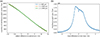 |
Figure 4 Simulation of position-, shape-, and size changes in the interference patch of a specimen near the Cat’s Eye reference position when translated. (a) Position of the interference’s patches center-of-gravity when moved perpendicular to the optical axis for three different axial distances. (b) Size of the interference patch when moved along the optical axis. |
The size and shape of the interference patch can also be used for pre-aligning the specimen to the Cat’s Eye reference position. Further away from the Cat’s Eye, the interference patch is a small rectangle that becomes larger, when the specimen is moved closer to the Cat’s Eye. In close proximity to the Cat’s Eye, the interference patch becomes circular and the interference fringe density decreases (compare Fig. 3b). In Figure 4b, the number of pixel corresponding to the area of the interference patch over its axial position is shown. The plateau in the center corresponds to the area, were the interference patch has a circular shape. This pre-alignment method can also be adapted for form measuring interferometers other than the TWI with different beam stop apertures as long as the aperture clipping is recognizable and related to the specimen position.
When the interferogram of the interference patch is evaluated using phase shifting interferometry, one can reconstruct the phase and from there the height values of the images. These values can then be compared to the values in the reference position. To investigate the influence of misalignment on these height value differences, several simulations of different positions close to the reference positions are performed and the height value differences are analyzed. To get insight into the relation between the form of the height value differences and the position of the specimen, the optical aberrations are expressed in terms of Zernike polynomials and the numbering of the coefficients follows the ISO/ANSI numbering convention [26, 27].
In Figure 5, the Zernike coefficients fitted to the height differences in dependence of the specimen’s position in relation to the Cat’s Eye reference position is shown. For this purpose, the height values resulting from a specimen at the specific position and the height values resulting from a specimen with it’s apex in the Cat’s Eye position are simulated and the results are subtracted from each other. The resulting difference wavefront is then developed into Zernike coefficients. In Figure 5a, the evolution of the Zernike coefficients from Z0 to Z20 ( to
to  in the double indexing scheme) are shown for an asphere that is moved along the optical axis. It can be seen that, apart from some changes in Z12 and Z14, the sweep is mainly affecting the so-called Defocus-aberration (Z4). The sweep along the optical axis was repeated with different specimens including the asphere, two spherical specimens with different radii, and a toroid. The Defocus over the axial position z is shown for them in Figure 5b. The linear region from |z − zCat’sEye| ≤ 300 μm corresponds to the region, where the interference patch of the specimen has its maximum area and a round shape. The zero-crossing of the Defocus is at zCat’sEye, which makes the Defocus a good criterion for the axial adjustment of the specimen into the Cat’s Eye reference position. It has to be noted that it is important to subtract the reference value simulated for the Cat’s Eye position to align the specimen position to the position used in the model. Otherwise, the adjustment by Defocus zero-crossing is less accurate and can have an offset. Figure 5c shows the Zernike coefficients of an asphere that is translated along lateral x-axis. Here, the coefficients of the primary x-Coma (Z8) appears to be affected the most. Therefore, in Figure 5d the change in Z8 over the lateral position is shown for the selected specimens. Again, the zero-crossing of the Coma appears at x = xCat’sEye and is therefore a good criterion for a coarse alignment along the x-axis. Simulations have further shown that the same can be achieved by primary y-Coma (Z7) for a coarse alignment along the y-axis. Note that the fine lateral alignment together with the alignment of tilt is performed in the final measurement position.
 |
Figure 5 Results of Zernike fit to the height difference values of position sweeps of simulated data for different specimens. (a) Zernike coefficients for an asphere moved along the optical axis. (b) Defocus-coefficient (Z4) for four different specimens over axial position. (c) Zernike coefficients for an apshere moved laterally. (d) Primary x-Coma for different specimens over lateral position. |
2.3 Position optimization algorithm
Following the simulations of the relation between the specimen’s position and the resulting interferogram, an algorithm for positioning the specimen in the Cat’s Eye reference position is introduced. The algorithm consists of three steps: First, a coarse positioning of the interference pattern to align the specimen’s apex with the optical axis is performed. Second, a coarse positioning along the optical axis is performed to the region, where the interferograms have a round shape. Finally, the positioning along the optical axis is optimized using the reconstruction of the height values and the minimization of the Zernike coefficients of the difference topography. All three steps are described in the following in detail.
For the coarse alignment of the specimen, the specimen is first manually brought into a position, where a rectangular interferogram of sufficient size is seen on the camera image. For the alignment, the center-of-gravity of the rectangular patch is calculated. First, to get the area of the interferogram, the image is blurred. This assures that the interference fringes in the rectangular patch are evened out and do not interfere with the estimation of the patch border. Second, the camera image is binarized by a threshold operation, dividing it into the bright region of the evened-out interference patch and the dark background. Afterwards, a contour finding operation [28, 29] is performed to find the perimeter of the interference patch. The center-of-gravity of the interference patch can then be calculated by dividing the first moment of the contour pixels by the zeroth moment along each lateral direction [30]. To align the specimen’s apex with the optical axis of the interferometer, the center-of-gravity of the rectangular patch has to be aligned with the interference patch position that corresponds with the optical axis. This position is estimated by the simulations described in Section 2.2. The difference vector between target position and the current center is calculated. Then the on-screen vector is translated to the movement of the specimen perpendicular to the optical axis using the previous simulation for estimating the translation factor. Afterwards, the center-of-gravity of the interference patch is estimated again and the calculation of the difference vector and the subsequent movement is repeated to refine the positioning and account for measurement inaccuracies and possible mismatch between simulation and real positioning. Usually now, the patch center matches the desired position within one or two pixels difference. With the simulations from Section 2.2 pixel shift of ±2 in patch center-of-gravity correspond to ±34 μm of specimen translation in lateral direction.
After this coarse lateral alignment of the specimen with the optical axis, the specimen is coarsely brought into the proximity of the Cat’s Eye reference position, which corresponds to the region of an enlarged circular interference patch as seen in Figures 3a and 3b. In this region, the Defocus and the primary x- and y-Coma are linear over the respective axial and lateral displacements (compare Figs. 5b and 5d). Since the area of the interference patch depends on the axial position, it can be used for determining the rough distance to the Cat’s Eye position and for bringing the specimen into the proximity. For this, the camera image is blurred and thresholded as before and the contour is calculated. Then, a floodfill operation inside the contour is performed and the number of pixels inside the contour is counted. With the data from the simulation shown in Figure 4b, the distance to the Cat’s Eye position can be estimated and the axial position of the specimen can be changed accordingly. Here, it is only important to get into the linear regime of the Defocus- and Coma-coefficients.
To deduce the Cat’s Eye reference position from the Defocus-coefficient of height values of the interferogram, the height values have to be calculated from the measurement data first. For this, the phase of the interferogram is retrieved by using 5 phase shifted interferograms. The reference arm of the TWI contains a phase-shifting element that is used to shift the angle of the reference phase in steps of  between φ1 = 0 and φ5 = 2π. The recorded intensity images I1 to I5 are then used with Hariharans phase reconstruction method [15] to retrieve the phase of the measured interferogram. In order to now get rid of the 2π-ambiguity of the phase image, phase unwrapping using the Goldstein method [16] is performed. The simulated height values of a specimen in the Cat’s Eye position are then subtracted from the height values measured. This ensures that the reference position for the real adjustment matches the simulation of the adjustment using the model of the TWI. The resulting height value differences are developed into Zernike polynomials. The Defocus-term (
 , [26]) of the Zernike developement is then a measure for the proximity of the specimen’s current position in relation to the Cat’s Eye reference position [20, 31]. The process of wavefront reconstruction and Zernike coefficient extraction is shown in Figure 6.
 |
Figure 6 Reconstruction process from phase shifted interference images including phase reconstruction, phase unwrapping with calculation of height values, subtraction of reference height values, and subsequent development into Zernike polynomials. |
Since the Defocus develops linearly near the Cat’s Eye reference position and has it’s zero-crossing directly at this position, several measurements and linear regression can be used to estimate the axial coordinate value. Therefore, the height values and the resulting Zernike-coefficients are repeatedly measured and the specimen is translated along the optical axis (z) between the measurements. In this particular case n = 5 measurements were performed and the specimen was moved by Δz = 75 μm between the measurements. Then, a linear regression of the estimated Defocus values was performed and the zero-crossing of the Defocus is calculated. The specimen is moved to this position and the height values are measured again. Since the lateral position in relation to the Cat’s Eye reference position has a linear relation to the primary x- and y-Coma ( and
and  ) the positioning perpendicular to the optical axis can be optimized here as well to achieve a coarse lateral alignment. In this case, both lateral coordinates (x and y) are optimized simultaneously by using the secant method, which is a special case of the Regula falsi [32]. The new value of x is given by
  with δx being the finite difference quotient defined as
  . The iterations of y follow in the same way. The first iteration from x0 to x1 and y0 to y1, respectively, use fixed steps Δx0 and Δy0 instead of
  and
and  . After a fixed number of iterations (here: n = 5), the position of the specimen perpendicular to the optical axis is refined sufficiently. After the lateral position optimization, the specimen might have moved and the distance between objective lens surface and the specimen’s surface measured along the optical axis might have changed. Therefore, the adjustment along the optical axis is refined by an additional optimization step. However, even if the lateral positioning was not performed, the refinement step is still applied to account for inaccuracies in the first axial optimization step. For this refinement, the current Defocus-value and the slope calculated previously in the linear regression step are used. This step can be repeated if necessary, since the slope might have changed slightly due to the lateral repositioning. The algorithm of the specimen positioning using the Zernike coefficients is shown in Figure 7.
 |
Figure 7 Scheme of the specimen positioning algorithm using the Zernike development of the height values reconstructed from the interference image. |
2.4 Repeatability of the Cat’s Eye positioning algorithm
For measuring the repeatability of the specimen positioning in the Cat’s Eye reference position, multiple specimens, containing spheres with different radii, aspheres, and freeform surfaces, are inserted into the TWI measurement setup and repeatedly brought into the reference position by the method described above. The final position along the optical axis is measured by a distance measuring interferometer (DMI) and the results are compared to reveal the spreading of the final position. The measurement setup is shown in Figure 8.
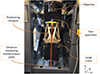 |
Figure 8 Measurement setup for surface measurements with the tilted-wave interferometer consisting of the interferometer itself (only objective shown), the specimen positioning system (large z-axis and positioning hexapod), the specimen, and the distance measuring interferometer. |
The setup consists of the TWI itself, from which only the objective is shown, the large z-axis with a positioning hexapod mounted on top, and a DMI below. The DMI measures the distance to the back of the positioning hexapod’s stage, were a retroreflector (PS975M-A, Thorlabs, Newton, NJ, USA) is mounted. Due to the limited beam displacement acceptance of the DMI, the lateral movement of the hexapod is limited to about ±0.5 mm until the DMI looses the measurement beam. The specimen is placed in a hydraulic chuck (05.043.258, GEWEFA Josef C. Pfister GmbH & Co. KG, Burladingen, Germany) in the center of the hexapod stage. The TWI objective has an assumed focal point of f = 48.609 mm, which resembles the distance between the last lens surface of the TWI objective and the Cat’s Eye reference position. The DMI (RLE10, Renishaw, Wotton-under-Edge, Gloucestershire, England, UK) uses a 90° sensor head (RLD10, Renishaw) and an environmental compensation unit (RCU10, Renishaw) with an air temperature sensor.
For the measurement of the repeatability of the adjustment of a specimen into the Cat’s Eye reference position, the specimen is inserted into the hydraulic chuck in the top stage of the positioning hexapod. The specimen is moved upwards in axial direction towards the estimated reference position until a rectangular interference patch of sufficient size appears on the camera image (compare Fig. 3). From here, a coarse lateral alignment of the specimen is performed using the center of gravity of the interference patch. Since this can lead to movements of the hexapod of more than 0.5 mm, this step is prone to the DMI loosing the reflected beam. The axial translation into the linear region of the Zernike developement of the height values follows, using data from the simulation as a lookup function. The main adjustment into the reference position uses the hexapod for the positioning. This algorithm can be performed with or without readjusting the lateral position of the specimen. For setting the reference position for the repeated measurements, an initial iteration of the positioning algorithm is performed. With the specimen in the Cat’s Eye position, the retroreflector is adjusted for optimal beam backreflection into the DMI. The specimen is then brought back to a starting position for the repetitions and the internal counter of the DMI is set to zero for marking this position as a reference position. From there, repeated adjustments into the Cat’s Eye position are performed with going back to the starting reference position after every iteration. To make sure that the algorithm performs reliably under different starting conditions, the starting position can be altered by a random offset in every iteration of the loop. The DMI value and the Zernike coefficients of the height values are recorded for every time that the Cat’s Eye position is reached.
3 Results and discussion
Repeated measurements with various test specimens were made following the process described above (Sect. 2.4). The utilized test specimens encompass an asphere [25], a toroidal surface [17] and two spherical test specimens (with radii of curvature R = 40 mm and R = 15 mm). Measurements both with and without lateral repositioning in the Cat’s Eye plane were performed and the DMI-value, the hexapod encoder values, and the Zernike coefficients from  up to
up to  were recorded. Since the DMI is prone to occasional glitches of the internal counter, a sufficiently long section of the data without glitch is selected to show the short term repeatability of the system. The reasons of the glitches and methods to reduce them will be investigated in future work. In Figure 9, repeated measurements for the Cat’s Eye adjustment along the optical axis without lateral repositioning can be seen for the four different test specimens.
 |
Figure 9 Measurement results of the repeated specimen adjustment into the Cat’s Eye reference position for four different specimens: (a) Axial position measured by DMI over measurement number with mean value subtracted. (b) Residual Defocus-coefficient over measurement number. |
The data in Figure 9a show a good short-term repeatability of the axial position measured with the DMI for the investigated specimens. The standard deviations are below 30 nm for all tested specimens. The individual values of the standard deviation σz are given in Table 1. In addition, the residual Defocus-values of the measurements shown in Figure 9b display standard deviations below 2 nm, hinting a good convergence of the positioning algorithm.
Results of the repeated specimen positioning measurements for the four tested specimens.
In addition to the repeatability of the axial position adjustment, the optional lateral position adjustment subsequent to the axial positioning was investigated with the test specimens described above in order to investigate, if the above described sensitivity of the Zernike coefficients primary x- and y-Coma to the lateral misalignment in the reference position is already large enough to achieve highly accurate lateral specimen positioning in this step. Since the DMI can only measure along the optical axis, the lateral position of the specimen is tracked by the axis encoders of the positioning hexapod. They don’t have the accuracy as the DMI, but are still good enough to estimate the lateral repeatability of this coarse alignment procedure. After each individual positioning, the axial position is resetted into a position showing a rectangular interference patch. In addition, the lateral position is changed by a random value between −50 m and 50 m for each axis to ensure that the centering works independent of the starting condition in a reasonable region. From the recorded positions for the repeated measurements the mean position is subtracted and the results for the four different test specimens are shown in Figure 10.
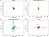 |
Figure 10 Repeated positioning of the test specimen along lateral axes (x and y) in the plane of the Cat’s Eye reference with mean value subtracted: (a) asphere, (b) sphere with radius 15 mm, (c) sphere with radius 40 mm, and (d) toroid. |
For the asphere and the sphere with the radius of 15 mm, the position measurements are densely packed around the mean position. However, for the larger sphere with 40 mm radius and for the toroid, the adjusted positions are more widely distributed. Especially for the larger sphere the positioning is rather unstable, leading to larger outliers. Here, the movement range during the positioning could be limited to prevent coarse misalignment. The standard deviation σx and σy of this positioning step are shown in Table 1. It can be seen that the positioning deviations are not equal for both axes, which may be caused by additional tilts of the specimens in the holder. This can be fixed by a subsequent fine alignment of the specimen in the measurement position. For estimating the resulting axial displacement from this lateral displacement, the measured deviations from the mean are used together with the design topography of the measured specimens. The point-wise axial offsets are calculated and ordered by magnitude. The highest offset of 95% of the data points (Δz95%(x, y)) is used as an estimate of the axial error due to lateral misalignment. For all but the sphere with radius 40 mm, the expected axial error Δz95% due to the lateral alignment is small against the axial error due to the axial adjustment σz. Using the design, one can estimate a maximum axial displacement due to the lateral displacement of about 4 nm. This error appears reasonably low. Nevertheless, these effects will be further minimized by the alignment correction, including both lateral specimen position and specimen tilt, in measurement position (which is much more sensitive to alignment errors), and respective repositioning of the Cat’s Eye. These next steps will be investigated in more detail in future work. It has to be further noted that the lateral displacement and the tilt of the specimen are parameters that are estimated during the surface reconstruction. This makes the measurement to a certain extent robust against alignment errors of these parameters.
In order to estimate the influence of the axial deviation of the specimen position from the Cat’s Eye position on the final form reconstruction, a virtual experiment was carried out: The maximum standard deviation of the axial position deviation of a specimen is estimated to σz ≈ 31 nm (27 nm for direct z-repeatability, compare Table 1, and 4 nm for the influence of the lateral misalignment). In a virtual experiment, the asphere was used as a test specimen and an axial misalignment of the specimen of twice the estimated standard deviation was used to simulate the measurement data. After form reconstruction from these simulated data, this results in a surface form reconstruction error of 4.5 nm RMS.
4 Conclusion
Surface alignment plays an important role in interferometric form measurement and misalignment can lead to measurement errors that are not obvious by the measurement results themselves. In tilted-wave interferometry, the form reconstruction results are especially sensitive to misalignment along the optical axis. Therefore, the accurate alignment of the specimen along the optical axis is crucial for a highly accurate form reconstruction.
In this work, we propose a specimen alignment procedure that uses the so-called Cat’s Eye reference position as an alignment reference and intermediate step for aligning the specimen into the measurement position. The Cat’s Eye position is a fixed position, independent from the measured specimen, where the focus of the interferometer’s optics and the apex of the measured specimen coincide. For aligning a specimen into this position, we show a three-step process: First, a pre-alignment of the specimen perpendicular to the optical axis, second, a rough alignment along the optical axis, and third, a fine alignment using the height values reconstructed from the interferogram. The last step aligns the specimen along the optical axis but can also be enhanced by a fine alignment perpendicular to the optical axis. From the reference position, the specimen can be transferred into the measurement position with the relative distance being tracked by a distance-measuring interferometer. This allows for a accurate positioning in relation to a fixed datum.
In a first step, the resulting camera images for different alignment steps, and the influence of different positioning steps and their sensitivities are investigated using simulations. From these insights, the Cat’s Eye adjustment procedure is developed and is then tested with the measurement setup and different specimens. The axial positioning shows a good short-term repeatability with a standard deviation in the range of between ≈15 nm and ≈30 nm. The fine-adjustment perpendicular to the optical axis depends on the chosen specimen but usually has only a small impact on the axial positioning accuracy. The overall impact of the positioning into the Cat’s Eye on the final form reconstruction result can be preliminary estimated to be around <5 nm RMS, but further investigations, including the transition to the measurement position have to be done.
Future work will focus on the positioning of specimens into the measurement position, which includes both the lateral position and the specimen tilt. After fine adjusting the lateral alignment in measurement position, the Cat’s Eye reference will be determined again in order to further reduce possible errors due to lateral misalignment. Then, the specimen is moved to the final measurement position and the surface form is reconstructed from the data acquired. This process will then be repeated several times, which would give insight into the overall repeatability of the measurement process. In addition, the absolute positioning accuracy of the specimen will be investigated: In a first step, well-known, calibrated reference specimens will be measured and the absolute form will be compared to reference values with well-known uncertainty. In a second step, the absolute position of the Cat’s Eye reference will be investigated utilizing an external white light interferometer to measure the distance between the top surface of a transparent test specimen and the last objective lens surface of the TWI. This would further enhance the matching between the digital twin of the TWI and the physical instrument and would therefore be a leap forward in understanding and improving the measurement uncertainty of the TWI.
Funding
This research has been supported by the Deutsche Forschungsgemeinschaft (grant no. 496703792).
Conflicts of interest
The authors declare that they have no competing interests to report.
Data availability statement
Data associated with this article cannot be disclosed due to legal reason.
Author contribution statement
Conceptualization, G.S. and I.F.; Methodology, G.S. and I.F.; Software, D.E. and G.S.; Validation, G.S. and I.F.; Formal Analysis, G.S.; Investigation, D.E. and G.S.; Resources, I.F.; Data Curation, D.E. and G.S.; Writing – Original Draft Preparation, G.S.; Writing – Review & Editing, I.F.; Visualization, G.S.; Supervision, I.F.; Project Administration, I.F.; Funding Acquisition, I.F.
References
- Hentschel R, Braunecker B, Tiziani HJ (Eds.), Advanced Optics Using Aspherical Elements (SPIE, 2008). ISBN 9780819467492. https://doi.org/10.1117/3.741689. [CrossRef] [Google Scholar]
- Rolland JP, Davies MA, Suleski TJ, Evans C, Bauer A, Lambropoulos JC, Falaggis K, Freeform optics for imaging, Optica 8, 161 (2021). https://doi.org/10.1364/OPTICA.413762. [NASA ADS] [CrossRef] [Google Scholar]
- Van Gestel N, Cuypers S, Bleys P, Kruth JP, A performance evaluation test for laser line scanners on CMMs, Opt. Lasers Eng. 47, 336 (2009). https://doi.org/10.1016/j.optlaseng.2008.06.001. [Google Scholar]
- Weckenmann A, Estler T, Peggs G, McMurtry D, Probing systems in dimensional metrology, CIRP Ann. 53, 657 (2004). https://doi.org/10.1016/S0007-8506(07)60034-1. [Google Scholar]
- Forman PF, The Zygo interferometer system, in Interferometry, vol. 0192, edited by GW Hopkins (1979), pp. 41–49. http://proceedings.spiedigitallibrary.org/proceeding.aspx?articleid=1229011. [Google Scholar]
- Knauer MC, Kaminski J, Hausler G, Phase measuring deflectometry: a new approach to measure specular free-form surfaces, in Optical Metrology in Production Engineering, vol. 5457, edited by W Osten, M. Takeda (2004), p. 366, ISSN 0277786X. https://doi.org/10.1117/12.545704. [Google Scholar]
- Beutler A, Metrology for the production process of aspheric lenses, Adv. Opt. Technol. 5, 211 (2016). https://doi.org/10.1515/aot-2016-0011. [Google Scholar]
- Kulawiec A, Murphy P, DeMarco M, Measurement of high-departure aspheres using subaperture stitching with the Variable Optical Null (VON), in 5th International Symposium on Advanced Optical Manufacturing and Testing Technologies: Advanced Optical Manufacturing Technologies, vol. 7655, edited by L. Yang, Y. Namba, D.D. Walker, S. Li, p. 765512 (2010). ISBN 9780819480859, ISSN 0277786X. https://doi.org/10.1117/12.864962. [Google Scholar]
- Küchel MF, Interferometric measurement of rotationally symmetric aspheric surfaces, Opt. Meas. Syst. Indust. Inspect. VI 7389, 389–422 (2009). https://doi.org/10.1117/12.830655. [Google Scholar]
- Greivenkamp JE, Gappinger RO, Design of a nonnull interferometer for aspheric wave fronts, Appl. Opt. 43, 5143 (2004). https://doi.org/10.1364/AO.43.005143. [Google Scholar]
- Garbusi E, Pruss C, Osten W, Interferometer for precise and flexible asphere testing, Opt. Lett. 33, 2973 (2008). https://doi.org/10.1364/OL.33.002973. [NASA ADS] [CrossRef] [Google Scholar]
- Baer G, Schindler J, Pruss C, Siepmann J, Osten W, Calibration of a non-null test interferometer for the measurement of aspheres and free-form surfaces, Opt. Express 22, 31200 (2014). https://doi.org/10.1364/OE.22.031200. [CrossRef] [Google Scholar]
- Schindler J, Baer G, Pruss C, Osten W, The tilted-wave-interferometer: freeform surface reconstruction in a non-null setup, in International Symposium on Optoelectronic Technology and Application 2014: Laser and Optical Measurement Technology; and Fiber Optic Sensors, vol. 9297, edited by J. Czarske, S. Zhang, D. Sampson, W. Wang, Y. Liao (2014), p. 92971. ISBN 9781628413830, ISSN 1996756X. https://doi.org/10.1117/12.2073053. [Google Scholar]
- Schachtschneider R, Stavridis M, Fortmeier I, Schulz M, Elster C, SimOptDevice: a library for virtual optical experiments, J. Sens. Sens. Syst. 8, 105 (2019). https://doi.org/10.5194/jsss-8-105-2019. [Google Scholar]
- Hariharan P, Oreb BF, Eiju T, Digital phase-shifting interferometry: a simple error-compensating phase calculation algorithm, Appl. Opt. 26, 2504 (1987). https://doi.org/10.1364/AO.26.002504. [Google Scholar]
- Goldstein RM, Zebker HA, Werner CL, Satellite radar interferometry: two-dimensional phase unwrapping, Radio Sci. 23, 713 (1988). https://doi.org/10.1029/RS023i004p00713. [Google Scholar]
- Fortmeier I, Stavridis M, Schulz M, Elster C, Development of a metrological reference system for the form measurement of aspheres and freeform surfaces based on a tilted-wave interferometer, Meas. Sci. Technol. 33, 045013 (2022). https://doi.org/10.1088/1361-6501/ac47bd. [CrossRef] [Google Scholar]
- Gronle A, Pruss C, Herkommer A, Misalignment of spheres, aspheres and freeforms in optical measurement systems, Opt. Express 30, 797 (2022). https://doi.org/10.1364/OE.443420. [Google Scholar]
- Fortmeier I, Stavridis M, Wiegmann A, Schulz M, Osten W, Elster C, Evaluation of absolute form measurements using a tilted-wave interferometer, Opt. Express 24, 3393 (2016). https://doi.org/10.1364/OE.24.003393. [CrossRef] [Google Scholar]
- Schmitz T, Evans C, Davies A, Estler W, Displacement uncertainty in interferometric radius measurements, CIRP Ann. 51, 451 (2002). https://doi.org/10.1016/S0007-8506(07)61558-3. [Google Scholar]
- Pruss C, Baer GB, Schindler J, Osten W, Measuring aspheres quickly: tilted wave interferometry, Opt. Eng. 56, 111713 (2017). https://doi.org/10.1117/1.OE.56.11.111713. [Google Scholar]
- Schindler J, Pruss C, Osten W, Increasing the accuracy of tilted-wave-interferometry by elimination of systematic errors, in Optical Measurement Systems for Industrial Inspection X, vol. 10329, edited by P. Lehmann, W. Osten, A. Albertazzi Gonçalves (2017), p. 1032904, ISBN 9781510611030, ISSN 1996756X. https://doi.org/10.1117/12.2270395. [Google Scholar]
- Schindler J, Pruss C, Osten W, Simultaneous removal of nonrotationally symmetric errors in tilted wave interferometry, Opt. Eng. 58, 1 (2019). https://doi.org/10.1117/1.OE.58.7.074105. [NASA ADS] [CrossRef] [Google Scholar]
- Baer G, Schindler J, Siepmann J, Pruß C, Osten W, Schulz M, Measurement of aspheres and free-form surfaces in a non-null test interferometer: reconstruction of high-frequency errors, Optical Measurement Systems for Industrial Inspection VIII, vol. 8788, edited by P.H. Lehmann, W. Osten, A. Albertazzi (2013), p. 878818. ISBN 9780819496041, ISSN 0277786X, https://doi.org/10.1117/12.2021518. [Google Scholar]
- Scholz G, Evers D, Fortmeier I, Influence of specimen positioning stage drift in tilted-wave interferometry for accurate form measurements for aspherical and freeform surfaces, in Optics and Photonics for Advanced Dimensional Metrology III, edited by P.J. de Groot, P. Picart, F. Guzman, vol. 12997, (SPIE, 2024), p. 42, ISBN 9781510673120. https://doi.org/10.1117/12.3017366. [Google Scholar]
- Thibos LN, Applegate RA, Schwiegerling JT, Webb R, Standards for reporting the optical aberrations of eyes, J. Refract. Surg. 18, 232 (2002). https://doi.org/10.3928/1081-597X-20020901-30. [Google Scholar]
- Niu K, Tian C, Zernike polynomials and their applications, J. Opt. 24, 123001 (2022). https://doi.org/10.1088/2040-8986/ac9e08. [NASA ADS] [CrossRef] [Google Scholar]
- Bradski G, The opencv library, Dr. Dobb’s J. Software Tools Profess. Program. 25, 120–123 (2000). [Google Scholar]
- Suzuki S, Be K, Topological structural analysis of digitized binary images by border following, Comput. Vis. Graph. Image Process. 30, 32 (1985). https://doi.org/10.1016/0734-189X(85)90016-7. [Google Scholar]
- Demtröder W, Experimentalphysik 1, Springer-Lehrbuch, 5th edn. (Springer Berlin Heidelberg, Berlin, Heidelberg, 2008), ISBN 978-3-540-79294-9. https://doi.org/10.1007/978-3-540-79295-6. [Google Scholar]
- Griesmann U, Soons J, Wang Q, DeBra D, Measuring form and radius of spheres with interferometry, CIRP Ann. 53, 451 (2004). https://doi.org/10.1016/S0007-8506(07)60737-9. [Google Scholar]
- Bronstein IN, Semendjajew KA, Musiol G, Mühlig H, Taschenbuch der Mathematik, 7th edn(Verlag Harri Deutsch, Frankfurt am Main, 2008), ISBN 978–3817120079. [Google Scholar]
All Tables
Results of the repeated specimen positioning measurements for the four tested specimens.
All Figures
|
Figure 1 Specimen positioning within the TWI. (a) Specimen positioned in the Cat’s Eye reference position. (b) Specimen moved to the measurement position, tracked by a distance-measuring interferometer (DMI). |
| In the text | |
|
Figure 2 (a) Optical setup of the TWI. (b) Example of four camera images with the sub-interferograms of an aspherical specimen created by the four mask positions of the microlens array. (c) Photo of the specimen stage of the TWI showing a specimen and the TWI objective. |
| In the text | |
|
Figure 3 Interferograms for a specimen (asphere) positioned in different positions around the Cat’s Eye reference position. (a) Sweep along the optical axis (z). (b) Sweep perpendicular to the optical axis (lateral sweep in x) in the plane of the Cat’s Eye position. (c) Sweep perpendicular to the optical axis in a plane 1 mm away from the Cat’s Eye position. |
| In the text | |
|
Figure 4 Simulation of position-, shape-, and size changes in the interference patch of a specimen near the Cat’s Eye reference position when translated. (a) Position of the interference’s patches center-of-gravity when moved perpendicular to the optical axis for three different axial distances. (b) Size of the interference patch when moved along the optical axis. |
| In the text | |
|
Figure 5 Results of Zernike fit to the height difference values of position sweeps of simulated data for different specimens. (a) Zernike coefficients for an asphere moved along the optical axis. (b) Defocus-coefficient (Z4) for four different specimens over axial position. (c) Zernike coefficients for an apshere moved laterally. (d) Primary x-Coma for different specimens over lateral position. |
| In the text | |
|
Figure 6 Reconstruction process from phase shifted interference images including phase reconstruction, phase unwrapping with calculation of height values, subtraction of reference height values, and subsequent development into Zernike polynomials. |
| In the text | |
|
Figure 7 Scheme of the specimen positioning algorithm using the Zernike development of the height values reconstructed from the interference image. |
| In the text | |
|
Figure 8 Measurement setup for surface measurements with the tilted-wave interferometer consisting of the interferometer itself (only objective shown), the specimen positioning system (large z-axis and positioning hexapod), the specimen, and the distance measuring interferometer. |
| In the text | |
|
Figure 9 Measurement results of the repeated specimen adjustment into the Cat’s Eye reference position for four different specimens: (a) Axial position measured by DMI over measurement number with mean value subtracted. (b) Residual Defocus-coefficient over measurement number. |
| In the text | |
|
Figure 10 Repeated positioning of the test specimen along lateral axes (x and y) in the plane of the Cat’s Eye reference with mean value subtracted: (a) asphere, (b) sphere with radius 15 mm, (c) sphere with radius 40 mm, and (d) toroid. |
| In the text | |
Current usage metrics show cumulative count of Article Views (full-text article views including HTML views, PDF and ePub downloads, according to the available data) and Abstracts Views on Vision4Press platform.
Data correspond to usage on the plateform after 2015. The current usage metrics is available 48-96 hours after online publication and is updated daily on week days.
Initial download of the metrics may take a while.