| Issue |
J. Eur. Opt. Society-Rapid Publ.
Volume 21, Number 2, 2025
|
|
|---|---|---|
| Article Number | 36 | |
| Number of page(s) | 15 | |
| DOI | https://doi.org/10.1051/jeos/2025025 | |
| Published online | 31 July 2025 | |
Research Paper
Image quality metrics for restricted gamut images produced by laser-induced printing on plasmonic films
1
Université Jean Monnet Saint-Etienne, CNRS, Institut d’Optique Graduate School, Laboratoire Hubert Curien UMR 5516, 42023 Saint-Etienne, France
2
TOPPAN Security SAS, 33 rue de Verdun, 92150 Suresnes, France
3
Institut Universitaire de France (IUF), Ministère de l’Enseignement Supérieur et de la Recherche, 1 rue Descartes, 75005 Paris, France
4
Inria, Domaine de Voluceau, 78150 Le Chesnay-Rocquencourt, France
* Corresponding author: This email address is being protected from spambots. You need JavaScript enabled to view it.
Received:
20
March
2025
Accepted:
19
May
2025
Abstract
Laser-induced printing is a low-cost, high-speed, non-contact method of marking large, high-resolution images. Implemented on thin films containing metallic nanoparticles, the technique allows for the printing of color images with visual effects. However, these images typically have a limited color gamut compared to inkjet printing. This limitation is due to the inability to achieve high levels of saturation for all colors and to cover the sRGB hue range. While common quality metrics focus primarily on aspects such as resolution or blur, they rarely address the color aspect. This study proposes a methodology to provide image quality metrics adapted to color gamuts with unusual shapes and volumes. It aims to rank them in terms of image quality performance for any given image. In particular, this work focuses on gamuts measured in transmission and reflection that are not necessarily centered on the CIE a*b* plane and may exhibit low contrast. Psychophysical studies have been conducted to evaluate the quality of images simulated with different color gamuts. The same images were evaluated using different metrics, and an analysis based on the ANOVA model was used to determine a set of metrics that explain observers’ preferences.
Key words: Image / Quality / Metrics / Laser Processing / Psychophysical / ANOVA
© The Author(s), published by EDP Sciences, 2025
 This is an Open Access article distributed under the terms of the Creative Commons Attribution License (https://creativecommons.org/licenses/by/4.0), which permits unrestricted use, distribution, and reproduction in any medium, provided the original work is properly cited.
Abbreviations
AIC: Akaike Information Criterion
AICc: a version of AIC, that has a correction for small sample size
IQA: Image Quality Assessment
IQM: Image Quality Metrics
MSE: Mean Squared Error
PSNR: Peak Signal to Noise Ratio
SSIM: Structure Similarity Index Measure
VIF: Variance Inflation Factor
1 Introduction
Recently, laser-induced colors on semi-transparent random plasmonic metasurfaces have enabled the first printing of multiplexed images observable to the naked eye under unpolarized white light [1]. These colors have the peculiarity of being independently controlled in different modes of observation. Indeed, two laser-processed areas can have the same color in one observation mode and different colors in another, while a single random plasmonic metasurface, i.e. a thin layer containing metallic nanoparticles that strongly interact with light, generates the colors. Thanks to this property, a multiplexed image can be encoded by laser processing in a single plasmonic metasurface and reveal different images in different observation modes. The versatility, speed and tamper-resistance of laser-induced image multiplexing make it an ideal laser-based technique for high-security documents personalization. However, the color gamut achievable with this method – and with laser printing method in general – is limited. For instance, in the work of Jiao Geng et al. (2022) [2], ultrafast laser processing was shown to produce structural colors with high resolution and durability, but the achievable color gamut remains limited to about 15% of the sRGB space and is highly dependent on the viewing angle. Similarly, Marek Mezera et al. (2023) [3] discussed how laser-induced periodic surface structures (LIPSS) can generate diffractive or plasmonic structural colors, but these methods struggle to reproduce a wide range of hues with high saturation.
Other studies further highlight these limitations. J. Bonse and S. Gräf (2021) [4] outlined several unresolved challenges in the fabrication of LIPSS, emphasizing the constraints in achieving a broad color range and practical scalability. S. Maragkaki et al. (2020) [5] investigated the influence of defects in LIPSS-generated structural colors, and found that such defects can cause color inconsistencies and further limit the achievable color gamut. In addition, S. Zhang et al. (2023) [6] investigated laser-written multilayer structural colors for full-color marking, but found that such techniques suffer from viewing angle limitations, making color perception inconsistent depending on the observer’s perspective.
As a result, these techniques cannot replicate the full range of colors accessible through standard printing techniques such as inkjet printing, where a wide color gamut is achieved using saturated cyan, yellow, magenta, and black primary inks [7].
Since the reference image often contains colors outside the achievable gamut, a gamut mapping step is necessary to adapt the printer reproduction to the constraints of the distorted gamuts. The gamut mapping process in this study is primarily based on the method proposed by Chosson and Hersch [8]. In this approach, primary colors – which include black, white and chromatic primaries – are first selected to define the target color gamut for the printing process. To account for differences in viewing conditions and ensure color consistency, a chromatic adaptation transform [9] is used. To preserve perceptual differences between light and dark areas, a lightness soft-compression is applied in [10], gently adjusting values to fit within the achievable range of our output medium. Gray axis alignment ensures that neutral tones remain consistent, preventing unwanted color casts in achromatic regions. Finally, chroma soft-compression is performed to maintain color saturation while keeping colors within the target gamut boundaries.
This structured approach enables effective gamut mapping, ensuring that source colors are accurately reproduced while maintaining visual consistency.
Due to the limited gamut of the laser-induced colors, traditional image quality metrics such as resolution, blur, and other Image Quality Assessment (IQA) criteria may prove inadequate for optimizing the laser printing process for color reproduction [11]. Several other metrics are commonly used in color reproduction studies that cover a range of characteristics. These include color [12–15], hue and chroma as defined by the CIE [16, 17], saturation [13, 15], color rendition [12, 18], processed color gamut [12], color reproduction [19], color shift [19, 20], gamut size [21], correctness of hue [22], and the proportionality of printed gamuts to their original counterpart [14]. In addition, perceptually driven metrics such as the Spatial Hue Angle MEtric (SHAME) [23] account for both spatial and color distortions, making them particularly relevant when evaluating color differences in constrained gamuts. However, the quality of the reproduction is markedly different when using the laser-induced gamut, which is considerably smaller and not centered around a grey axis in comparison to the typical printer gamuts referenced in the literature.
The aim of this study is to identify appropriate objective metrics for assessing the image quality of color images reproduced by laser processing with a limited color gamut. A one-way Analysis of Variance (ANOVA) [24, 25] method was conducted in conjunction with an Akaike Information Criterion (AIC) model selection test [26, 27] to determine which objective metrics are most appropriate for estimating the subjective IQA. These metrics will guide the optimization of laser parameters to enhance image quality or to compare color gamuts produced by various materials or laser parameter sets.
Given the large number of possible laser parameter combinations and the inherent difficulty in predicting their effect on color, an empirical approach is required. This approach involves laser printing millions of metasurfaces using a wide range of laser parameters and then measuring them in different observation modes. Once the colors have been measured, they are used to simulate images with different laser-induced gamuts corresponding to different types of initial random plasmonic metasurfaces and different observation modes. The challenge of ensuring optimal observation modes for each observer on different real samples for classification purposes led us to conduct a survey on digital images. The simulated images were evaluated on a monitor by human observers, who reported normal or corrected-to-normal vision in an uncontrolled viewing environment on their personal computer, using comparison rather than absolute color evaluation to mitigate the effect of viewing condition variability. The observers were asked to classify the images, which had been simulated with different gamuts being given the reference of the image obtained with a sRGB gamut. They were asked to do this based on how faithful to the original the reproductions appeared to them.
In Section 2, we introduce the foundations of image quality analysis, define image quality, review existing metrics, and present our approach for extracting a final metric from established methods. Section 3 details the subjective image quality assessment (IQA) conducted, including the survey setup, gamuts and images used. In Section 4, we present the results of our analysis and propose a new objective metric aligned with the subjective ratings. Finally, the conclusion discusses the strengths and limitations of our approach, along with perspectives for future improvements and applications.
2 Material and methods
Image quality can be defined as the assessment by human observers of the visual elements that make an image pleasing to them [28]. The main factors that affect image quality are noise, blur, and color reproduction.
Since images are one of the most common methods of conveying information, whether in digital or physical documents, it is of the utmost importance to create the most satisfying images possible with the available means, emphasizing the need for metrics to evaluate them.
To obtain information about image quality, human judgments are required to perform a subjective IQA which is then averaged over all the results since observers have different standards. In the literature, objective evaluation methods are categorized as full-reference, reduced-reference or no-reference methods [29]. The full-reference method consists in comparing a degraded image with its original (reference), these difference methods can be performed:
-
Pixel-by-pixel, using metrics like CIEDE2000 color difference formula or the ΔUCS if performed in the OSA-UCS space [30];
-
Based on the structure of the image, with metrics such as the Structure Similarity (SSIM) Index or Visual Information Fidelity [31];
-
Based on perception, using metrics like the Visual Difference Predictor (VDP).
Reduced-reference methods rely on only a portion of the reference image, while utilizing the full information of the degraded image to compute the quality metrics. No-reference methods are based on metrics without any reference image at all, such as the Blind/Reference less Image spatial Quality Evaluator (BRISQUE) or the Naturalness Image Quality Evaluator (NIQE) [32]. In the present study, the distortion of the laser-induced gamuts, relative to the sRGB gamut, necessitated the addition of a reference image to prevent the observers’ aesthetic and color preferences from dominating in the quality assessment.
As mentioned in the introduction, objective IQA can be conducted using a large variety of metrics. Accordingly, the one-way ANOVA method was used to identify the most relevant objective IQA metrics compared to subjective IQA. One-way ANOVA is a statistical technique used to compare the means of three or more independent groups to determine if there is a statistically significant difference between them. It assumes that the groups are normally distributed with equal variances. The method calculates the F-statistic, which is the ratio of the variance between the group means to the variance within the groups. A significant F-statistic suggests that at least one group means differs significantly from the others, which may require further post hoc analysis to pinpoint the differences.
In evaluating the relevance of metrics within a linear model, one-way ANOVA is a useful tool for determining whether different metrics, treated as categorical variables, lead to significant differences in the model’s performance. It is important to understand the effect of individual parameters to explain observations. For example, Jost-Boissard et al. [33] used the one-way ANOVA to investigate whether there was a link between observer characteristics (skin type, age, gender and expertise) and their appreciation of different light sources. By applying one-way ANOVA, significant effects of changes in these metrics on the model’s output can be assessed, thereby identifying which metrics are most influential. This approach ensures that the final model remains both efficient and interpretable by focusing on metrics that significantly contribute to explain the model.
Coupling this method with Akaike Information Criterion (AIC) can yield the most promising models that ensure strong predictive performance while avoiding overfitting. AIC is a method for comparison and selection models in statistical modeling, it is based on the trade-off between the goodness of fit of the model and its complexity. It is defined as: (1)where k is the number of parameters in the model, and L is the maximum likelihood of the model. Lower AIC values indicate a model that better balances fit and complexity, making it preferred over models with higher AIC values. The AIC penalizes models with more parameters, thus helping to avoid overfitting.
When evaluating the relevance of metrics within a linear model, AIC can be used to compare different models that include different sets of metrics. By calculating the AIC for each model, the combination of metrics that results in the most parsimonious model – one that provides a good fit with minimal complexity – can be identified. This method is particularly useful in model selection, where the goal is to retain only the most relevant metrics that contribute to the model’s predictive power while avoiding unnecessary complexity. The purpose of this study is to evaluate the quality of the plasmonic colors presented on a sample by establishing the IQA. While the laser-induced colors on semi-transparent random plasmonic metasurfaces are promising for many applications, such as image multiplexing, the colors produced tend to be less saturated and not centered within the color gamut when compared to those of a CMYK inkjet printer. As a result, a tailored IQA approach is required to accurately evaluate their reproduction quality. To better understand the characteristics of the tested samples, Figure 1 shows the back side of a sample with a semi-transparent plasmonic metasurface deposited on the front side. The colored areas were produced by laser processing [1]. The sample is illuminated by an LED panel (4000 K, 350 lm) and observed in specular reflection. The transmitted light is reflected by a black mirror positioned beneath the sample. The black mirror was used to balance the amount of transmitted and reflected light from the sample, making it possible to observe color areas in both reflection and transmission modes on a single photograph. The image illustrates the potential of laser-induced gamut generation on a specific random plasmonic metasurface, showing the achievable colors in two distinct observation modes. Such samples and setup allow to record color datasets pertaining to a single observation mode and sample, with each color area associated with a distinct laser parameter set. Each data set corresponds to a distinct color gamut.
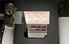 |
Figure 1 Photograph of a sample illuminated from the back side with a semi-transparent laser-processed plasmonic metasurface on the front side. The colors exemplify two laser-induced gamuts observed in reflection and transmission modes on a single sample. |
Six gamuts were utilized to generate a series of images for ranking by human observers. The first three ones, displayed in Figures 2a–2c were directly built from the colors of laser-processed random plasmonic metasurfaces measured in the back side reflection mode on three different samples:
-
1_BR corresponds to a low chromaticity gamut (C* below 20) but presents colors of all different hues (h*), its lightness values (L*) are between 20 and 60.
-
6_BR corresponds to a gamut with low lightness contrast (L* between 25 and 55) and presents a chromaticity value (C*) of up to 40, however only in the yellow domain (yellow hue h*).
-
8_BR shows a higher gamut volume than the two previous ones, has chromaticity values (C*) up to 40 and lightness values (L*) ranging from 20 to 80, but is really centered around yellow and presents no achromatic color with high lightness.
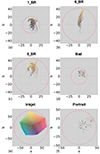 |
Figure 2 Six gamuts used for the study presented in the CIE a*b* color plane with luminance color code. (a-c) correspond to laser-processed metasurfaces observed in back side reflection. (d) represents a synthetic small gamut. (e) represents a full color gamut of an inkjet printer without the black ink. Figure (f) represents a gamut which colors are extracted from a portrait image. |
On the other hand, Figure 2d shows a synthetic gamut designed to produce images of poor quality (named Bad). This gamut was constructed by randomly selecting 50 primaries using NumPy’s uniform random generator within specified ranges: lightness values (L*) between 40 and 60, and chromaticity values (a*, b*) ranging from −2 to 20. This approach resulted in a non-centered gamut with low chromaticity (C*), allowing to verify whether the question about image quality is well understood by observers since this gamut should be ranked last for the majority of cases. Figure 2e illustrates the gamut of a CMY inkjet printer simulated using a Yule-Nielsen color prediction model calibrated with 36 printed color patches (named Inkjet). This gamut exhibits a wide range of colors, extending to high chromaticity (a*, b*) values in all directions, but lacks contrast with lightness (L*) values, none of which being below 40. Figure 2f illustrates a gamut consisting of colors extracted from a portrait image (named Portrait). A set of 100 primaries within the convex hull of the gamut was selected to create this color palette. This figure corresponds to a high-contrast, low-color gamut, with lightness (L*) ranging from 15 to 90, and chromaticity (a*, b*) going as high as 50, but only in the red/orange region, which is closest to skin tones.
Twenty-four different images were utilized for the subjective IQA based on questionnaires. Each image was reproduced using the six selected gamuts described above and sent through a survey for ranking by the observers on their personal display. In order to reduce the influence of the image content on the quality rating of the images to be assessed, our study included images representing various cases (see Fig. 3). Eight portrait images (Figs. 3a–3d) and (Figs. 3i–3l) were presented on a neutral background, similar to that found on identity documents. These images showed individuals with different skin tones. Among other images, some show a colorful content whose main colors can be inferred due to their spatial distribution (e.g. Fig. 3e). Some others have a colorful content whose main colors can hardly be inferred from their spatial distribution (e.g. Fig. 3f). Some images were selected because of their dull colors, or because their gamut is mainly located in one hue sector such as Figure 3w with only green colors. The image shown in Figure 3u is black and white and serves as a contrast and white achromaticity checker. The preliminary colorfulness evaluation of each image was performed using the Hasler colorfulness metric [34], and the resulting values are presented in Table 1.
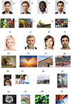 |
Figure 3 Images used for the subjective IQA. |
The simulated images that were presented with the question format (Appendix A) to the observers for image quality evaluation were generated by employing a gamut mapping algorithm [1, 8] on the original image, as described in the introduction. This algorithm maps the colors present in the original image to the available gamut. Some gamut being highly restricted, this gamut mapping algorithm contains a gray axis alignment [8], as well as a color adaptation step [4], which distinguishes it from conventional gamut mapping algorithms, such as CARISMA [11], GCUSP [11], SKNEE [35] or WCLIP [36].
The assessment of image preferences was carried out through the implementation of an uncontrolled psychophysical experiment. The observers were presented with 24 times the same question wherein 6 images were reproduced using the 6 selected gamuts, the observers were also presented the original image in full color. Participants in the psychophysical experiments included 34 individuals (whose age range was 20–65 years old, and who were either junior college students or lab/company workers). Every observer had at least some background in either color science or image processing with either formal studies or being frequently exposed to laser-printed images, four of them could even be considered experts. All participants reported normal or corrected-to-normal vision. The experiments were conducted remotely using the participants’ personal computers. While no standard calibration was enforced, participants were instructed to perform the experiment in a well-lit room without direct glare on the screens and to avoid extreme ambient lighting. All observers used their computer rather than their mobile phone, whose resolution is assumed to be at least 1920 × 1080. To mitigate viewing variability, relative comparisons (rather than absolute color judgments) were used throughout the test design. The observers were asked to rank the images from 1 to 6, with 1 representing the closest match to the original image and 6 the least faithful reproduction according to them. The observers utilized their own display devices and were instructed to ensure that the night filter was disabled and that the screen exhibited sufficient luminosity. As the images were ranked in relative order and not absolute order there was no need to use color calibrated displays.
3 Results
A total of 34 observers participated in this experiment, from nine different countries, primarily in Europe. The distribution of answers is illustrated in the histograms presented in Figure 4. This figure displays 24 histograms, each corresponding to 1 of 24 images presented in Figure 3. Each histogram depicts, along the y axis, the number of individuals who ranked the image simulated with each gamut (corresponding to different colors) from “rank 1” to “rank 6”. The x-axis represents the rank assigned to each simulated image. The pink bar is for the portrait gamut, cyan for the printer one, purple for the bad one, orange for “1_BR”, green for “6_BR” and “8_BR” for the red one. The height of each color segment within a bar reflects the number of observers who assigned that particular gamut to the given rank, making it possible to visualize ranking tendencies across images.
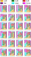 |
Figure 4 Distribution of preference rankings for each image ((a)–(x)) from Figure 3 based on the overall ranking. The x-axis represents the assigned rank, and the y-axis indicates the number of observers who assigned each rank. |
As evidenced by the histograms, the question posed was effectively understood by the observers. The intentionally bad gamut was consistently ranked last by a large majority of observers, indicating that there were no inversions in ranking. In all observations, no responses were identified as anomalous, indicating that filtering was unnecessary. This was confirmed by the Z-score method [37], which filters all values exceeding two standard deviations from the mean, and did not change the results. Furthermore, as illustrated in Figure 4, the experimental gamuts appear to perform better than the intentionally bad gamut, and worse than the printer and portrait gamuts for almost all observers.
With respect to the ranking from the observers (Fig. 4), the portrait gamut is ranked first for the portrait images (Figs. 3a–3d, 3i–3l), in accordance with expectation, as well as for images (3g, 3o–3u), exhibiting a Hasler colorfulness value of less than 0.25 as shown in Table 1. In the case of images exhibiting a Hasler colorfulness exceeding 0.25, the printer gamut is preferred by observers, despite its lower contrast, as evidenced by the responses to images 3e and 3h. The results are less conclusive for the three experimental gamuts (orange, green and red bars) that the observers ranked between ranks 3 and 5, with a ranking rarely occurring in the same order.
A previous study, available in the Supplementary Information section, was also conducted to determine how observers assessed colorfulness and contrast in addition to ranking images based on their preference. This was done with the images (a)–(h) only without the reference image being given. Regarding the colorfulness criterion, previous observations indicated that the observers’ ability to assess colorfulness was influenced by the inherent colorfulness of the original image. While highly colorful images facilitated clearer differentiation between gamuts, less colorful images led to more ambiguous rankings. On the contrary, contrast assessment appeared to be more consistent across all image types, suggesting that contrast variations were more perceptible to observers regardless of the image’s initial characteristics.
These findings motivated the inclusion of a colorfulness metric in the present model to ensure that the relationship between perceived image quality and gamut characteristics could be more effectively captured. These findings also highlighted the need to include a metric for categorizing large color hue shifts, as this can lead to discrepancies between objective colorfulness and subjective preference. Indeed, while certain gamuts may exhibit higher colorfulness and contrast, excessive color shifts could reduce their perceived quality, meaning that colorfulness and contrast metrics alone would be far from being sufficient.
However, while some images may appear to favor one gamut over the other, this preference is not consistently evident when all images are considered together.
4 Discussion
In this section, twenty objective metrics, listed in Table 2, were selected to evaluate the quality of each simulated image. The value of each metric was calculated for the 144 simulated images corresponding to the 24 original images (Fig. 3) simulated using the 6 gamuts of Figure 2. Linear regression analysis, performed using RStudio, was employed to estimate the coefficients linking the objective metrics to the observer-based rankings.
List of the twenty metrics considered.
Among the selected objective metrics, some were gamut dependent only, while others depended on both the original image and the gamut. All of them were normalized between 0 and 1 in order to ensure the comparability of the coefficients within a linear model. The normalization was done using the formula: (2)
(2)
For instance, the convex hull area metric was normalized by setting the minimum possible value to 0 and the maximum possible value to the area of the convex hull of the gamut in the a*b* plane, ensuring that the normalization process is independent of the image or gamut set used.
Before performing an ANOVA analysis of the metrics used, the dataset was first categorized based on the Hasler colorfulness of the original images. This allows to separate the data into two groups, high and low colorfulness, to ensure that the differences in image color characteristics were accounted for. Then, different linear models were applied to each group, rather than using a single model for the entire data set, to better capture potential variations in behavior across different levels of colorfulness.
In order to find the optimal colorfulness threshold, several values were tested to find out how to split the data set. This threshold was also compared to some arbitrary random groups. To compare these splits, the R2 value was computed on the expected rank vs. actual rank of the final models, then the most satisfying R2 values were selected.
The final R2 values for the different splitting cases are shown in Table 3. The threshold value of 0.2 was chosen because it yielded the best R2 value of 0.973 for the final model, which is also higher than those obtained by random splitting. Hereafter, the “low colorfulness group” and “high colorfulness group” refer to the sets of rankings and corresponding metrics derived from images with a Hasler colorfulness below 0.2 and above 0.2, respectively.
Optimal split for threshold tuning.
The observer rankings were approximated by linearly correlating the objective metrics with the rankings. The Variance Inflation Factor (VIF) [40] was utilized to deal with multicollinearity, where metrics are highly correlated with each other. Metrics with high VIF values, indicating a strong correlation with other metrics, were considered redundant and were excluded from the model. In this case, M14 and M15 metrics were highly correlated.
After removing redundant metrics, the linear regression was recalculated to derive the final coefficients. It was computed for both the low and high colorfulness groups. To assess the importance of each metric in predicting rankings, a one-way ANOVA was performed (Table 4). ANOVA partitions the total variance in the observer rankings into components attributable to each metric, providing insight into the relative importance of each metric. Specifically, the ANOVA test compares the variance explained by each metric to the residual variance to determine which metrics contribute significantly to the model.
Coefficients found for the 19 metrics analyzed with the ANOVA.
For this analysis, the probability of a Type I error “alpha” was set at 0.1, meaning that a metric was considered significant when there was less than a 10% probability that the effect of the metric was due to chance. The p-value is a statistical measure that indicates the likelihood of getting the same results if there is no effect. Metrics with a p-value below 0.1 were identified as key predictors. These metrics were then used to create various models, each representing a different linear combination of the significant metrics. The Akaike Information Criterion (AIC) was used to determine the best model. AIC evaluates each model by considering both the goodness of fit and the number of parameters, favoring simpler models that adequately explain the data. Due to the limited sample size, the corrected AIC (AICc) was used, which adjusts the AIC for small sample sizes, ensuring a more accurate model selection.
The AICc model analysis shown that the metrics listed in Table 5 were the most promising since they showed p-values below 0.01.
Metrics kept for each group indicated with a cross.
The linear regression used with a simplified prediction model, as a linear combination of M4, M9, M3 and M5 for the low colorfulness group, gives: (3)
(3)
And the linear combination of M4, M9, M11, M16 and MSE for the low colorfulness group yields: (4)
(4)
These predictions give an overall R2 value of 0.873. However, Figure 5 shows that there are 3 populations of points: one with the two best gamuts, the printer and portrait gamuts, one with the experimental gamuts, and one with the bad gamut.
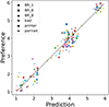 |
Figure 5 Ranking resulting from the subjective IQA evaluation (Pref) vs predicted ranking based on equations (3) and (4) (Pred). The colors correspond to the different images. |
Figure 6 displays six simulated images from the original image (a) of Figure 3, with their subjective ranking compared with the ranking predicted by equations (3)/(4). It shows how well the metric is able to discriminate the artificial good and bad gamuts from the experimental, but there is still confusion to rank the experimental gamuts reproduction.
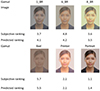 |
Figure 6 Simulated images with the six gamuts and comparison of predicted and subjective rankings. |
To address the observed ambiguity in subjective rankings across experimental gamuts mainly, a plot of the actual and predicted ranks is shown in Figure 7. In this figure, vertical error bars represent a ±0.7 rank tolerance which was the average standard deviation among the observers’ ranking for the experimental gamuts. This threshold accounts for minor perceptual differences that may not be reliably distinguished by observers. Points whose error bars intersect the diagonal (y = x) are marked in green, indicating that the predicted ranking falls within an acceptable range of the true subjective rank. This visual representation highlights that 138 out of 144 (and 69 out of 72 for experimental gamuts) misalignments are minor and localized.
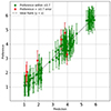 |
Figure 7 Actual and predicted ranks for each image. |
To further assess the consistency between the predicted and actual subjective rankings, a confusion matrix (Fig. 8) was introduced using the ordinal ranks of each gamut per image. This representation makes it easier to visualize correct matches and mismatches between predicted and observer-derived rankings. For 15 out of the 24 tested images, all six gamuts were ranked in the same order as those provided by human observers. Among the remaining cases, the mismatches were limited to close gamuts, suggesting localized ambiguity rather than a broader failure in prediction. Notably, these discrepancies primarily stemmed from confusion between two gamuts that often received similar rankings. Appendix D shows the observer ranking variability in the case of a difficult to rank image.
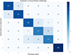 |
Figure 8 Confusion matrix between actual and predicted ranks for all images. |
The comparison of the average rank of the gamuts for all images and the average prediction is shown in Table 6.
Predicted and subjective ranking for each gamut averaged over the 24 images.
As it looks in Table 6, while the metrics do not always perfectly distinguish the best gamut among the actual gamuts, they still reveal meaningful patterns. This aligns with the observed variability in subjective rankings, where the standard deviation was notably high for the experimental gamuts.
The proposed linear models were initially calibrated for reflective structural gamuts; the generalization potential of these models to other imaging systems requires further consideration. While the current models provide an effective framework for reflective displays, their applicability to emissive or transmissive displays would need to be re-evaluated, especially in cases where the perceptual weighting of metrics may differ between systems, despite the models being robust to low variability on observers ranking (Appendix E).
The key metric most likely to be affected by a change in illuminant is the “Distance from the selected white point to the image gamut” (M16). This metric quantifies how a shift in the illuminant alters the perceived white point in the color palette, which is essential for evaluating color reproduction under varying lighting conditions and across different display technologies. Therefore, the applicability of the linear models should be reassessed when considering such changes in illuminant, ensuring their robustness in diverse imaging contexts.
The metrics seems to be usable for transmission mode colors for the samples to some degree as shown in Appendix B.
This metric has the interest of being linked not only to the gamut used for printer reproduction but also to the original image considered.
5 Conclusion
In this study, we established a relationship between several objective metrics from the literature and a subjective IQA of images simulated with different color gamuts using an observer-ranked method.
The relative consistency of the study results suggests that the observers had a clear understanding of the ranking protocol, but some difficulties to rank experimental gamuts that have different kinds of limitations. We identified a combination of metrics that efficiently differentiate printer reproduction quality when the variations are sufficiently pronounced. However, the model’s performance proved less reliable for experimental gamuts, as participants encountered difficulties ranking these reproductions despite having access to the original image, highlighting the inherent subjectivity of the task.
Moving forward, this approach could be extended to other observation modes, as the colors studied here correspond to the ones printed by a laser-induced printer on transparent plasmonic films, observed on backside reflection mode, which are significantly different than those on transmission and frontside reflection modes. Adding observers’ data from images simulated on those modes could add some robustness to the model. The results of this study, along with the extracted metrics, provide valuable insight into selecting the most suitable gamut for printing a given image. This, in turn, contributes to a better understanding of gamut quality and its impact on the final printer reproduction.
Acknowledgments
The authors thank the observers for giving their time for this research by answering the surveys.
Funding
This work is funded by the ANR project SLICID (ANR-23-CE39-0006).
Conflicts of interest
The authors have nothing to disclose.
Data availability statement
The data from the survey, as well as the intermediate metrics calculation results are available at https://github.com/robmermillod/IQM-Data/.
Author contribution statement
Conceptualization, Alain Tremeau and Nathalie Destouches; Methodology, Alain Tremeau, Aldi Wista Fadhilah, and Nathalie Destouches; Software, Robin Mermillod-Blondin and Aldi Wista Fadhilah; Formal Analysis, Robin Mermillod-Blondin, Nicolas Dalloz, Rémi Emonet, and Nathalie Destouches; Validation, Alain Tremeau; Writing – Original Draft Preparation, Robin Mermillod-Blondin and Nicolas Dalloz; Review & Editing, Alain Tremeau, Nicolas Dalloz, Rémi Emonet and Nathalie Destouches; Supervision, Nathalie Destouches.
Supplementary material
Figure S1: First set of color images considered.
Figure S2: Distribution of preference rankings for each image (a) – (h) from Figure S1 based on the overall image quality. The x-axis represents the assigned rank, and the y-axis indicates the number of participants who assigned each rank.
Figure S3: Distribution of ranks for each image (a) – (h) from Figure 7, based on colorfulness.
Figure S4: Distribution of contrast rankings for each image (a) – (h) from Figure 8 based on contrast.
Figure S5: Prediction vs Preference for FR results.
Figure S6: Prediction vs Preference for Transmission mode results.
Table S1: Hasler colorfulness values of images shown in Figure S1.
Access Supplementary MaterialReferences
- Dalloz N, et al., Anti-counterfeiting white light printed image multiplexing by fast nanosecond laser processing, Adv. Mater. 34(2), 2104054 (2022). https://doi.org/10.1002/adma.202104054. [Google Scholar]
- Geng J, Xu L, Yan W, Shi L, Qiu M, High-speed laser writing of structural colors for full-color inkless printing, Nat. Commun. 14, 565 (2023). https://doi.org/10.1038/s41467-023-36275-9. [Google Scholar]
- Mezera M, Florian C, Willem RG, Krüger J, Bonse J, Creation of material functions by nanostructuring, in: Ultrafast laser nanostructuring: the pursuit of extreme scales, edited by Stoian R, Bonse J (Springer International Publishing, Cham, 2023), p. 827–886. https://doi.org/10.1007/978. [Google Scholar]
- Bonse J, Gräf S, Ten open questions about laser-induced periodic surface structures, Nanomaterials, 11(12), 3326 (2021). https://doi.org/10.3390/nano11123326. [Google Scholar]
- Maragkaki S, et al., Influence of defects on structural colours generated by laser-induced ripples. Sci. Rep. 10, 53 (2020). https://doi.org/10.1038/s41598-019-56638-x. [Google Scholar]
- Zhang S, et al., Laser writing of multilayer structural colors for full-color marking on steel, Adv. Photon. Res. 5(1), 2300157 (2024). https://doi.org/10.1002/adpr.202300157. [Google Scholar]
- Baumann E, Hofmann R, Schaer M, Print performance evaluation of ink jet media: Gamut and Dye Diffusion, J. Imaging Sci. Technol 44(6), 500–507 (2000). [Google Scholar]
- Chosson SM, Hersch RD, Color gamut reduction techniques for printing with custom inks, in: Color imaging: device-independent color, color hardcopy, and applications VII (SPIE, 2001). https://doi.org/10.1117/12.452980. [Google Scholar]
- Zhai Q, Luo MR, Study of chromatic adaptation via neutral white matches on different viewing media, Opt. Express, 26, 7724–7739 (2018). https://doi.org/10.1364/OE.26.007724. [Google Scholar]
- Choi B, Hu S, Guo R, He W, He D, Chiu GT, Allebach JP, Developing a gamut mapping method for a novel inkjet printer, Color Imaging: Displaying, Processing, Hardcopy, and Applications, 2841–2846 (2022). [Google Scholar]
- Morovič J, To develop a universal gamut mapping algorithm, PhD Thesis, University of Derby, 1998. [Google Scholar]
- Dalal EN, Rasmussen DR, Nakaya F, Crean PA, Sato M, Evaluating the overall image quality of hardcopy output, in: PICS 1998: IS&T’s 1998 Image Processing, Image Quality, Image Capture, Systems Conference, Portland, Oregon, USA, May 17–20, 1998. [Google Scholar]
- Bonnier N, Schmitt F, Brettel H, Berche S, Evaluation of spatial gamut mapping algorithms, in: Color and imaging Conference 14, 56-61 (Society of Imaging Science and Technology, 2006). [Google Scholar]
- Hardeberg JY, Bando E, Pedersen M, Evaluating colour image difference metrics for gamut‐mapped images, Color. Technol. 124(4), 243–253 (2008). [Google Scholar]
- Lin C, Mottaghi S, Shams L, The effects of color and saturation on the enjoyment of real-life images, Psychon. Bull. Rev. 31, 361–372 (2024). https://doi.org/10.3758/s13423-023-02357-4. [Google Scholar]
- Internationale Beleuchtungskommission, ed., Colorimetry, 3rd ed., Publication/CIE No. 15 (Comm. Internat. de l’éclairage, 2004). [Google Scholar]
- Morovic J, Sun PL, Visual differences in colour reproduction and their colorimetric correlates, in: Color and Imaging Conference (Vol. 10, pp. 292-297), (Society of Imaging Science and Technology, 2002). [Google Scholar]
- Gast G, Tse MK, A report on a subjective print quality survey conducted at Nip16. In: Nip & Digital Fabrication Conference, Soc. Imaging Sci. Technol. 2001(2), 723–727 (2001). [Google Scholar]
- Miyata K, Tsumura N, Haneishi H, Miyake Y, Subjective image quality for multi-level error diffusion and its objective evaluation method, J. Imaging Sci. Technol. 43(2), 170–177 (1999). [Google Scholar]
- Norberg O, Westin P, Lindberg S, Klaman M, Eidenvall L, A comparison of print quality between digital and traditional technologies, in: Proc. IS&T-SID DPP2001: International Conference on Digital Production Printing and Industrial Applications, Antwerp, Belgium, 2001. [Google Scholar]
- Andersson M, Norberg O, Color gamut: Is size the only thing that matters?, in: TAGA 2006 (TAGA, 2006), p. 273. [Google Scholar]
- Hunt RWG, The reproduction of colour (John Wiley & Sons, 2005). ISBN: 0-470-02425-9. [Google Scholar]
- Pedersen M, Bonnier N, Hardeberg JY, Albregtsen F, Attributes of image quality for color prints, J. Electron. Imaging 19, 011016 (2010). https://doi.org/10.1117/1.3277145. [Google Scholar]
- Montgomery DC, Design and Analysis of Experiments (John Wiley & Sons, 2017). [Google Scholar]
- Hocking RR, Methods and applications of linear models: regression and the analysis of variance, John Wiley & Sons, 2013). [Google Scholar]
- Wagenmakers EJ, Farrell S, AIC model selection using Akaike weights, Psychon. Bull. Rev. 11(1), 192–196 (2004). https://doi.org/10.3758/bf03206482. [Google Scholar]
- Burnham KP, Anderson DR, Model selection and inference. A practical information–theoretic approach (Springer-Verlag, Heidelberg, 1998). https://doi.org/10.1007/978-1-4757-2917-7_3. [Google Scholar]
- Burningham N, Pizlo Z, Allebach JP, Image quality metrics, Encyclopedia Imaging Sci. Technol. 1, 598–616 (2002). https://doi.org/10.1002/0471443395.img038. [Google Scholar]
- Khan MU, Luo MR, Tian D, No-reference image quality metrics for color domain modified images. J, Opt. Soc. Am. A 39, B65–B77 (2022). https://doi.org/10.1364/josaa.450595. [Google Scholar]
- Simone G, Oleari C, Farup I, An alternative color difference formula for computing image difference, in: Proceedings from Gjøvik Color Imaging Symposium, 2009. [Google Scholar]
- Sheikh HR, Bovik AC, Image information and visual quality, IEEE Trans. Image Process. 15(2), 430–444 (2006). https://doi.org/10.1109/TIP.2005.859378. [Google Scholar]
- Eldarova EL, Starovoitov VA, Iskakov KA, Comparative analysis of universal methods no reference quality assessment of digital images, J. Theor. Appl. Inf. Technol. 99(9), 1977–1987 (2021). [Google Scholar]
- Jost-Boissard S, Avouac P, Fontoynont M, Preferred color rendition of skin under LED sources, LEUKOS: The J. Illuminating Eng. Soc. North America 12(1–2), 1–15 (2016). https://doi.org/10.1080/15502724.2015.1060499. [Google Scholar]
- Hasler D, Suesstrunk SE, Measuring colorfulness in natural images, in: Human Vision and Electronic Imaging VIII, Vol. 5007, edited by Rogowitz BE, Pappas TN (SPIE, Santa Clara, CA, 2003), pp. 87–95. https://doi.org/10.1117/12.477378. [Google Scholar]
- Braun GJ, A Paradigm for color gamut mapping of pictorial images, Thesis, Rochester Institute of Technology, 1999. Accessed from https://repository.rit.edu/theses/2860. [Google Scholar]
- Sun PL, Morovic J, What differences do observers see in colour image reproduction experiments? Conference on Colour in Graphics, Imaging and Vision 1, 181–186 (2002). https://doi.org/10.2352/cgiv.2002.1.1.art00040. [Google Scholar]
- Rousseeuw PJ, Hubert M, Robust statistics for outlier detection, WIREs Data Min & Knowl 1, 73–79 (2011). https://doi.org/10.1002/widm.2. [Google Scholar]
- Rigau J, Feixas M, Sbert M, An information-theoretic framework for image complexity, in: Proceedings of the First Eurographics Conference on Computational Aesthetics in Graphics, Visualization and Imaging, Girona, Spain, 2005, pp. 177–184. [Google Scholar]
- Houser KW, Wei M, David A, Krames MR, Whiteness perception under LED Illumination, LEUKOS 10, 165–180 (2014). https://doi.org/10.1080/15502724.2014.902750. [Google Scholar]
- Akinwande MO, Dikko HG, Samson A, Variance inflation factor: as a condition for the inclusion of suppressor variable(s) in regression analysis, Open J. Stat. 05, 754 (2015). https://doi.org/10.4236/ojs.2015.57075. [Google Scholar]
Appendix A: Explanation given to the participants
You are invited to participate in our image quality assessment experiment. In this experiment, people will be asked to rank several batches of reproduction of the same image using different gamut. You will be given the original image and asked to rank different reproductions on how good they look to you compared to the others. This is an uncontrolled experiment that can therefore be done under any viewing and lighting condition. The experiment should take approximately 20 minutes to complete. Your participation in this study is completely voluntary. There are no foreseeable risks associated with this project. However, if you feel uncomfortable answering any questions, you can withdraw from the experiment at any point. Your experimental responses will be strictly confidential and data from this research will be reported only in the aggregate. Your information will remain confidential.
You will be asked to rank the six reproductions displayed based on how well they represent the original image.
You have to drag the image on the right panel: on top the one you deemed is the best reproduction and, on the bottom, the one you deemed the worst (Fig. A1). It is only based on your preference. This ranking is subjective and there is no “right” or “wrong” answer.
 |
Figure A1 Question asked by the experimenter. |
Thank you very much for your time and support.
Appendix B: Metrics tested on previous transmission data
Here, the metric provided in equations (3) and (4) is used to predict the preference of observers for the 8 images provided in Figure S1 (see Supplementary Information) with the gamuts being:
-
Portrait is the same
-
Bad is the same
-
Printer is adapted to transmission mode as well using Yule-Nielsen model and has way lower lightness
-
3 gamuts in transmission
Figure B1 shows the preference vs prediction graph. The metric is doing decent at separating experimental gamut but ranks the printer gamut too positively despite the lightness being low. The R2 value here is 0.83, which is better than the 0.76 value of R2 provided by the modeled specifically designed for this question and presented in Supplementary Information Figure S6.
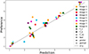 |
Figure B1 Preference vs prediction ranks for all images. |
Appendix C: Metrics dispersion for experimental gamuts
Figure C1 presents the disparity of metrics for the 3 experimental gamuts and for 4 images. The images used for this graph are (c) and (o) for low colorfulness images, (m) and (x) for high colorfulness images. For each metric represented in the horizontal axis, there are 4 sub-columns each representing from left to right image (c), (m), (o) and (x), in each of those sub-columns there are 3 dots representing the values for each of the 3 experimental gamuts. It appears that the most spread metrics are on M11, M16 and MSE, which are not the main ones. M4 and M9 are more useful to distinguish the synthetic gamuts from the rest.
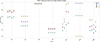 |
Figure C1 Metrics dispersion for experimental gamuts. |
Appendix D: Observers answer dispersion for two types of images
Figure D1 presents the dispersion of the observer ranking for images (c), which seems to have been ranked in the same order by a majority of observers, and image (x), which raised more uncertainty.
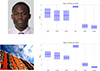 |
Figure D1 Observers rank dispersion. |
Appendix E: Robustness of the model to variations in observer ranking
To assess the robustness of the model to small variations in observer rankings a supplementary analysis simulating plausible sources of uncertainty has been conducted.
Controlled noise has been added to participant responses by randomly swapping adjacent ranks. Specifically, for each observer and each image, a 20% probability to swap rank 1 and 2, rank 2 and 3, and so forth was applied. This stochastic perturbation aimed to model intra-observer inconsistencies without drastically altering the underlying preference structure.
To evaluate the impact of these variations, the R2 value between the prediction and preference ranking by the observers in these cases was computed for 10 independent runs. This variation in the observer ranking led to a R2 variation of about 0.0031 with a standard deviation of 0.0004, which led to a decrease in model R2 from 0.973 to about 0.942. This result suggests that the model retains relatively high performance even when faced with moderate inconsistencies in observer data.
All Tables
All Figures
|
Figure 1 Photograph of a sample illuminated from the back side with a semi-transparent laser-processed plasmonic metasurface on the front side. The colors exemplify two laser-induced gamuts observed in reflection and transmission modes on a single sample. |
| In the text | |
|
Figure 2 Six gamuts used for the study presented in the CIE a*b* color plane with luminance color code. (a-c) correspond to laser-processed metasurfaces observed in back side reflection. (d) represents a synthetic small gamut. (e) represents a full color gamut of an inkjet printer without the black ink. Figure (f) represents a gamut which colors are extracted from a portrait image. |
| In the text | |
|
Figure 3 Images used for the subjective IQA. |
| In the text | |
|
Figure 4 Distribution of preference rankings for each image ((a)–(x)) from Figure 3 based on the overall ranking. The x-axis represents the assigned rank, and the y-axis indicates the number of observers who assigned each rank. |
| In the text | |
|
Figure 5 Ranking resulting from the subjective IQA evaluation (Pref) vs predicted ranking based on equations (3) and (4) (Pred). The colors correspond to the different images. |
| In the text | |
|
Figure 6 Simulated images with the six gamuts and comparison of predicted and subjective rankings. |
| In the text | |
|
Figure 7 Actual and predicted ranks for each image. |
| In the text | |
|
Figure 8 Confusion matrix between actual and predicted ranks for all images. |
| In the text | |
|
Figure A1 Question asked by the experimenter. |
| In the text | |
|
Figure B1 Preference vs prediction ranks for all images. |
| In the text | |
|
Figure C1 Metrics dispersion for experimental gamuts. |
| In the text | |
|
Figure D1 Observers rank dispersion. |
| In the text | |
Current usage metrics show cumulative count of Article Views (full-text article views including HTML views, PDF and ePub downloads, according to the available data) and Abstracts Views on Vision4Press platform.
Data correspond to usage on the plateform after 2015. The current usage metrics is available 48-96 hours after online publication and is updated daily on week days.
Initial download of the metrics may take a while.