© The Author(s), published by EDP Sciences, 2026

1 Introduction

Structured light has attracted strong interest in recent years, largely driven by its wide range of applications and by rapid progress in generating and detecting tailored optical fields [1, 2]. Within this area, partially coherent sources are increasingly regarded not as a limitation but as a useful degree of freedom, since the engineering of spatial coherence can mitigate drawbacks of highly coherent beams. Recent reviews emphasize that partially coherent beams with structured coherence have been explored for concrete applications including: optical imaging [3, 4], free-space optical communications with improved robustness to atmospheric turbulence [5–8], coherence-based optical encryption and robust signal/information transmission through complex or scattering media [8, 9], optical manipulation [10, 11], and remote sensing [12]. These are some of the reasons why there is great interest in devising, realizing, and characterizing new light sources, both coherent and partially coherent, that allow the characteristics of the light radiated by these sources to be modified in a controlled way [13–38].

Interesting and promising results are derived from the presence of phase vortices, which confer unique capabilities to the beam radiated from the source [5, 6, 12, 39–54]. For example, they find application in optical manipulation, because they can exert torque on microscopic particles, enabling advanced optical tweezers and micromanipulation [10, 46]; in imaging and metrology, where they offer new possibilities for super-resolution or phase-sensitive detection [12, 44]; in optical communication, since they provide an extra degree of freedom, the orbital angular momentum (OAM), for multiplexing and increasing data capacity [5, 6]. Vortex beams are typically generated using elements such as spiral phase plates, computer-generated holograms, q plates, or metasurfaces that encode the desired OAM mode [47, 50, 51, 53].

Recently, a new type of partially coherent light source, namely, a source with uni-variable cross-spectral density (CSD), has been proposed [38]. The peculiarity of sources of this class is that their CSD [55] can be directly derived from a function of a single complex variable [38]. The only requirement this function has to fulfill in order for it to be associated with a well-defined CSD is that its Taylor expansion must involve only non-negative coefficients. Several analytical forms, in some cases very simple, of bona-fide CSD can be devised in this way. Sources with uni-variable CSD are defined within a finite circular region, related to the convergence domain of the above Taylor series, and can be expressed as the superposition of coherent modes [55] carrying optical vortices. The analytical form of the vortex modes is quite simple, both across the source plane and in the far zone, enabling the study of the coherence features of the source, as well as those of the field radiated under Fraunhofer conditions [38]. One of the important features of univariable CSDs is their capability to customize at will the contributions from various coherent modes, serving, at the same rate, as the OAM modes. This renders them ideal for high-capacity information-transfer applications employing structured light.

The main aim of the present paper is, on one hand, to extend to the Fresnel regime the study of the propagation of beams radiated from sources with uni-variable CSD; on the other hand, to study the effects of truncating the number of the modes involved in the expansion. Examples will be presented concerning the so-called sZegö source, introduced in [38], which is obtained with an infinite number of Taylor terms, all with the same coefficient. Taking only a finite number of terms gives rise to the truncated sZegö source, introduced here, which represents a more realistic model for a partially coherent source, suitable to be physically realized. Finally, hints for devising other types of uni-variable CSDs are given for some cases in which the CSD takes a simple closed form.

2 Preliminaries

2.1 Uni-variable CSDs

A uni-variable CSD [38] is defined from any function g of a single complex variable ζ such that:$$g\left(\zeta \right)=\sum _{n=0}^{\infty }\mathrm{}{c}_n{\zeta }^n,$$(1)where$$c_n\ge 0 (\forall n),$$(2)and ζ belongs to the convergence domain of the series. By suitably scaling the argument of g it is always possible to set such a domain as$$\left|\zeta \right|<1.$$(3)

The CSD associated with g is obtained by letting$$\zeta =\frac{r_1{r}_2}{r_0^2}{e}^{i({\phi }_1-{\phi }_2)},$$(4)where (r₁, φ₁) and (r₂, φ₂) are the polar coordinates of two points across the source plane ( r ₁ and r ₂ ) and r₀ is the radius of the circular region where the source is defined. It should be noted that although the CSD depends on two points, for this class of sources, the dependence enters only through the single complex parameter ζ, following the terminology introduced previously in reference [38]. Therefore, using equations (1) and (4) we define, across the plane z = 0,$$W\left({\mathit{r}}_{\mathbf{1}},{\mathit{r}}_{\mathbf{2}},0\right)=g\left(\frac{r_1{r}_2}{r_0^2}{e}^{i\left({\phi }_1-{\phi }_2\right)}\right)=\sum _{n=0}^{\infty }\mathrm{}{c}_n{\left(\frac{r_1{r}_2}{r_0^2}\right)}^n{e}^{\mathrm{in}\left({\phi }_1-{\phi }_2\right)},\hspace{1em}\left(\right|r|<r_0).$$(5)

The sum in equation (5) can be read as the Mercer expansion of W₀, that is, [55]$$W({\mathit{r}}_{\mathbf{1}},{\mathit{r}}_{\mathbf{2}},0)=\sum _{n=0}^{\infty }\mathrm{}{\lambda }_n{\mathrm{\Phi }}_n({\mathit{r}}_{\mathbf{1}},0){\mathrm{\Phi }}_n^{\mathrm{*}}({\mathit{r}}_{\mathbf{2}},0),$$(6)with coherent modes (taking into account their normalization) given by$${\mathrm{\Phi }}_n(\mathit{r},0)=\sqrt{\frac{n+1}{\pi r_0^2}}{\left(\frac{r}{r_0}\right)}^n\mathrm{circ}\left(\frac{r}{r_0}\right)e^{\mathrm{in\phi }},\hspace{1em}(n=\mathrm{0,1},...),$$(7)and eigenvalues$${\lambda }_n=c_n\frac{\pi r_0^2}{n+1},\hspace{1em}(n=\mathrm{0,1},...),$$(8)where circ(r) is the characteristic function of a unit disk centered at the origin of the axes. The second argument of the modes Φ_n refers to the z-coordinate of the transverse plane where they are evaluated (in this case, across the source, that is, z = 0). The condition in equation (2), together with equation (8), guarantees that λ_n  > 0 (∀n), so that the CSD turns out to be well defined [13, 14].

The modes in equation (7) are recognized at once as optical vortices [49] with charge n. They have the same structure as Laguerre–Gaussian beams [56] in which the Laguerre polynomial has order zero and where the Gaussian function has been replaced by a circ.

The number of genuine CSDs that can be obtained following the present approach is practically unlimited, the only constraint that the function g has to fulfill being the fact that the coefficients of its Taylor expansion are all non-negative. Examples will be given in the following, where simple forms of CSDs will be presented, together with the mean features of the beams they radiate.

2.2 Characterization of uni-variable CSDs in OAM space

Uni-variable CSD represents one of a few known model optical fields that carry OAM in multiple modes, either finite or infinite. For the characterization of radial-only correlations among the OAM modes in such fields, the coherence–orbital angular momentum (COAM) matrix $\stackrel{\text{⃡}}{W}({\rho }_1,{\rho }_2,z)$ and its derivatives can be used [57]. Each element of the COAM matrix is a scalar radial field correlation at a pair of OAM indices, given by the expression:$$W_{\mathcal{l}m}\left(r_1,r_2,z\right)=\frac{1}{4{\pi }^2}\underset{0}{\overset{2\pi }{\int }}\mathrm{}\underset{0}{\overset{2\pi }{\int }}\mathrm{}W\left(r_1,r_2,z\right)e^{-i\left(\mathcal{l}{\phi }_1-m{\phi }_2\right)}\mathrm{d}{\phi }_1\mathrm{d}{\phi }_2,\hspace{1em}-\infty <\mathcal{l},m<\infty .$$(9)

The COAM matrix is the counterpart of the CSD matrix defined in polarization space to the OAM space and carries similar properties (quasi-Hermiticity, non-negative definiteness, etc.). However, it can have any size, say L × L, where L is the largest by magnitude OAM index involved. Also, for theoretical models, infinitely dimensional matrices are possible with certain convergence constraints. The uni-variable beam model is of this type.

Two derivatives of the COAM matrix are important and will be considered here. First, the OAM degree of coherence is the analog of the EM degree of coherence in the OAM space [58]:$$o(r_1,r_2,z)=\frac{\sqrt{\mathrm{Tr}\left[{\stackrel{\text{⃡}}{W}}^{†}\right(r_1,r_2,z\left)\stackrel{\text{⃡}}{W}\right(r_1,r_2,z\left)\right]}}{\prod _{j=\mathrm{1,2}}\mathrm{}\sqrt{\mathrm{Tr}\stackrel{\text{⃡}}{W}(r_j,r_j,z)}}.$$(10)

It provides the cumulative information about the normalized correlations at a pair of radii for all pairs of the OAM modes, regardless of the OAM phase information contained in each mode.

Second, it was found that a harmonic beam carrying OAM in L modes traces an orbitalization ellipse in LD OAM space (polar Fourier space) at a fixed radius [59], analogously to the two/three component electric field tracing a polarization ellipse in real 2D/3D space. To extend this geometric description to partially coherent beams, the COAM matrix can be considered at a single radius r₁ = r₂ = r, and regarded as the L × L orbitalization matrix [60]:$$\stackrel{\text{⃡}}{O}(r,z)=\stackrel{\text{⃡}}{W}(r,r,z),$$(11)the term steaming from its formal similarity to a polarization matrix. In LD the orbitalization matrix is shown to decompose into three parts: completely orbitalized, unorbitalized, and partially orbitalized, in which mixing occurs for mode couples, triples, …, up to L − 1. The completely orbitalized matrix is shown to factorize, representing a beam indistinguishable from harmonic, and, hence, described by an orbitalization ellipse. The contribution of the intensity of the completely orbitalized portion of the beam in the total beam, at a fixed radius, was introduced as the degree of orbitalization [60]:$$O(r,z)=\frac{{\sigma }_0(r,z)-{\sigma }_1(r,z)}{\sum _{n=0}^{\infty }\mathrm{}{\sigma }_n(r,z)},$$(12)where σ₀(r, z) ≥ σ₁(r, z) ≥ … ≥ σ_L(r, z) ≥… is the ordered sequence of the eigenvalues of $\stackrel{\text{⃡}}{O}$, all being real and nonnegative due to its Hermiticity and non-negative-definiteness. This quantity is analogous in nature to the degree of polarization and reduces to it in form for L = 2 and 3. In this work, we will thoroughly examine its behavior for uni-variable beams.

We note that for a univariable CSD the COAM matrix is diagonal and hence the calculations of both derivatives are relatively simple. For example, the OAM DOC becomes$$o(r_1,r_2,0)=\frac{\sqrt{\sum _{n=0}^{\infty }\mathrm{}{c}_n^2(r_1{r}_2/r_0^2{)}^{2n}}}{\prod _{j=\mathrm{1,2}}\mathrm{}\sqrt{\sum _{n=0}^{\infty }\mathrm{}{c}_n(r_j/r_0{)}^n}}.$$(13)

As we show below, for uni-variable beams σ₀ and σ₁ may depend on different c_n at different radii and, hence, it appears impossible to write down an explicit single formula for the degree of orbitalization. Instead, a piecewise-continuous function will be used, with its interval endpoints determined numerically.

3 Beams radiated by uni-variable CSDs

The propagation from sources with uni-variable CSD, both in the near and in the far field, can be dealt with starting from their expansion in terms of coherent modes. In such a way, from equation (6) we have, at any plane z = const.,$$W({\mathit{r}}_{\mathbf{1}},{\mathit{r}}_{\mathbf{2}},z)=\sum _{n=0}^{\infty }\mathrm{}{\lambda }_n{\mathrm{\Phi }}_n({\mathit{r}}_{\mathbf{1}},z){\mathrm{\Phi }}_n^{\mathrm{*}}({\mathit{r}}_{\mathbf{2}},z),$$(14)where the expression of the propagated modes Φ_n( r , z) depends on the approximation we use.

Using the expression above, the spectral density and the degree of coherence of the radiated field can be evaluated as [55]$$S(\mathit{r},z)\equiv W(\mathit{r},\mathit{r},z)=\sum _{n=0}^{\infty }\mathrm{}{\lambda }_n{\left|{\mathrm{\Phi }}_n(\mathit{r},z)\right|}^2,$$(15)and$$\mu ({\mathit{r}}_1,{\mathit{r}}_2,z)\equiv \frac{W({\mathit{r}}_1,{\mathit{r}}_2,z)}{\sqrt{S({\mathit{r}}_1,z) S({\mathit{r}}_2,z)}},$$(16)respectively.

3.1 Coherent modes in paraxial regime

Within the paraxial approximation, the propagation of the modes can be studied through the Fresnel integral, which, for a typical field V(r, φ, z), in polar coordinates reads [55]$$V(r,\phi ,z)=-\frac{\mathrm{ik}{\mathrm{e}}^{\mathrm{i}\mathrm{kz}}}{2\pi z}\underset{0}{\overset{\infty }{\int }}\mathrm{}\underset{0}{\overset{2\pi }{\int }}\mathrm{}V(\mathrm{r\text{'}},\phi \text{'},0)e^{i\frac{k}{2z}\left[{\mathrm{r\text{'}}}^2+r^2-2\mathrm{r\text{'}r}\cos (\phi \text{'}-\phi )\right]}\mathrm{r\text{'}}\mathrm{d}\mathrm{r\text{'}}\mathrm{d}\phi \text{'}.$$(17)

Using the equality$$J_n\left(t\right)=\frac{1}{2\pi }\underset{0}{\overset{2\pi }{\int }}\mathrm{}{e}^{\mathrm{in\psi }-\mathrm{it}\sin \psi }\mathrm{d}\psi ,$$(18)after some manipulations the propagated modes take the following form:$${\mathrm{\Phi }}_n(\mathit{r},z)=\frac{2N_F}{r_0}\sqrt{\pi (n+1)}{e}^{\mathrm{ikz}}(-i{)}^{n+1}\times e^{\mathrm{in\phi }}{e}^{\mathrm{i\pi }{N}_F{\rho }^2}{\int }_0^1\mathrm{}{J}_n(2\pi N_F\rho u)e^{\mathrm{i\pi }{N}_F{u}^2}{u}^{n+1}\mathrm{d}u,$$(19)where the Fresnel number has been introduced as$$N_F=\frac{k{r}_0^2}{2\pi z},$$(20)together with the normalized transverse coordinate$$\mathit{\rho }=\frac{\mathit{r}}{r_0}=(\xi ,\eta ).$$(21)

It is seen that the vortex structure of the phase is preserved during propagation and that, once the order n has been set, the propagated field depends only on the Fresnel number, as happens for the diffraction of a plane wave by a circular hole (corresponding to n = 0) [61]. Therefore, the Fresnel number will be taken as the natural variable to represent the propagation distance. As examples, density plots of the spectral density of some modes across the plane (x, z), that is, the squared modulus of the expression in equation (19), are shown in Figure 1.

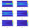Fig. 1 Density plots of the spectral density of some modes, |Φn ( r , z)|2, across the plane (ξ, z) for n = 0, 1, 2, 3, 4, 5.

As a first remark, we note that the property for a CSD of being uni-variable across a certain plane is not preserved during propagation. In fact, when modes propagate, their analytical forms actually change, and, in general, the product of the propagated modes, ${\mathrm{\Phi }}_n({\mathit{r}}_1,z) {\mathrm{\Phi }}_n^{\mathrm{*}}({\mathit{r}}_2,z)$, is no longer proportional to $r_1^n{r}_2^n\exp \left[\mathrm{in}\right({\phi }_1-{\phi }_2\left)\right]$, as it is required for the series to be interpreted as a power expansion.

Second, as also appears from Figure 1, the on-axis irradiance is zero for all modes, except n = 0. Furthermore, the modes spread during propagation at a rate that increases with n, giving less and less significant contributions in the central zone of the transverse planes. In particular, we expect that, when superpositions of modes are considered, only a finite number of modes need to be taken into account, which depends on the extent of the region where the field has to be evaluated. For example, modes with order 5 or higher can be safely neglected if the field has to be evaluated at N_F  = 0.5 within a circular region of radius 2r₀ (see Fig. 1).

3.2 Coherent modes in the far field

Unlike mode propagation in the Fresnel regime, far-field conditions lead to simple analytical forms. When the Fraunhofer conditions are met, the expression of a typical field (say, V_∞ ) is obtained from the Fourier transform, suitably scaled, of the field across the source [61]. For simplicity, the coordinate across the Fourier plane (say ν ) will be taken as the spatial coordinate across a transverse plane in the far zone. Disregarding unessential proportionality factors and curvature terms, we simply write$$V_{\infty }\left(\mathit{\nu }\right)=\iint \mathrm{}V(\mathit{r},0)e^{-2\pi i\mathit{\nu }\cdot \mathit{r}}\mathrm{d}\mathit{r},$$(22)the integral extending over the whole z = 0 plane.

Using polar coordinates, the above integral reads$$V_{\infty }\left(\mathit{\nu }\right)={\int }_0^{\infty }\mathrm{}{\int }_0^{2\pi }\mathrm{}V(r,\phi ,0)e^{-2\pi \mathrm{i\nu }r\cos (\vartheta -\phi )}r\mathrm{d}r\mathrm{d}\phi ,$$(23)

with ν and ϑ being the polar coordinates of ν . For the case of the modes in equation (7), the above integral gives$${\mathrm{\Phi }}_{n,\infty }\left(\mathit{\nu }\right)=\frac{2(-i{)}^n}{r_0}\sqrt{\pi (n+1)}{e}^{\mathrm{in\vartheta }}{\int }_0^{r_0}\mathrm{}{\left(\frac{r}{r_0}\right)}^{n+1}{J}_n\left(2\pi \nu r\right)\mathrm{d}r,$$(24)

J_n being the Bessel function of the first kind and order n [62]. Exploiting the following relation obeyed by the Bessel functions [63]:$$\begin{array}{l}\frac{\mathrm{d}}{\mathrm{d}\eta }\left[{\eta }^{n+1}{J}_{n+1}\left(\eta \right)\right]={\eta }^{n+1}{J}_n\left(\eta \right),\end{array}$$(25)the expression of the modes propagated in the far zone takes the simple form$${\mathrm{\Phi }}_{n,\infty }\left(\mathit{\nu }\right)=2r_0(-i{)}^n\sqrt{\pi (n+1)}{e}^{\mathrm{in\vartheta }}\frac{J_{n+1}\left(2\pi r_0\nu \right)}{2\pi r_0\nu }.$$(26)

Note that for n = 0 the latter equation gives rise to the well-known Fraunhofer diffraction pattern from a circular hole [61]. Indeed, for n = 0 the vortex field coincides with that of an ordinary plane wave. For n ≠ 0, we can read equation (26) as the diffraction pattern produced by a vortex field that impinges on a circular aperture [48].

Plots of the spectral density of the propagated modes of equation (26) are given in Figure 2 for n = 5, 10, 15. It appears that, in general, the function is very small until its argument reaches values roughly equal to n, and then slowly goes to zero in an oscillating way.

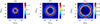Fig. 2 Plots of the spectral density of the modes in the far field, equation (26) for n = 5 (a), 10 (b), 15 (c), with r0 = 1.

In light of the above result, it is useful to express the CSD of a beam radiated by a uni-variable source through its Mercer expansion, which reads$$W_{\infty }({\mathit{\nu }}_1,{\mathit{\nu }}_2)=4\pi r_0^2\sum _{n=0}^{\infty }\mathrm{}{\lambda }_n(n+1)e^{\mathrm{in}({\vartheta }_1-{\vartheta }_2)}\frac{J_{n+1}\left(2\pi r_0{\nu }_1\right)}{2\pi r_0{\nu }_1}\frac{J_{n+1}\left(2\pi r_0{\nu }_2\right)}{2\pi r_0{\nu }_2}.$$(27)

In some cases, this expression even leads to closed forms for the degree of coherence in the far field (μ_∞). This happens, for example, if λ_n ∝ (n + 1) and we limit ourselves to point along radial directions (i.e., ϑ₁ = ϑ₂), in which case it can be shown that [64]$${\mu }_{\infty }({\nu }_1,\vartheta ,{\nu }_2,\vartheta )=2\frac{J_1\left(2\pi r_0({\nu }_1-{\nu }_2)\right)}{2\pi r_0({\nu }_1-{\nu }_2)}.$$(28)

4 sZegö and truncated sZegö sources

The first example of a uni-variable CSD we are going to show is that of the so-called sZegö source. The features of such a source across the source plane and in the far zone were studied and commented on in detail in a previous paper [38]. Here, we limit ourselves to recalling some of the main results obtained there. The effects of paraxial propagation of the radiated field will be studied here on the basis of the expression of the propagated modes obtained in Section 3.1. However, we find it convenient to perform such an analysis starting from a different uni-variable CSD, namely, the truncated sZegö CSD. Unlike sZegö CSD, in fact, the latter requires a finite number of modes and reduces to sZegö CSD when the number of modes goes to infinity. In such a way, the propagation features of the beams they radiate can be evaluated exactly through finite sums. However, we want to stress that a CSD of this type is interesting in itself because it is suitable to be synthesized in the laboratory starting from the superposition of a finite number of coherent fields [20, 28, 32, 37].

4.1 The sZegö source

To obtain a sZegö CSD we let c_n = I₀(∀n) in equation (1), with I₀ a positive constant having dimensions of irradiance, so that$$g\left(\zeta \right)=\frac{I_0}{1-\zeta }\left(\left|\zeta \right|<1\right),$$(29)and the corresponding CSD turns out to be$$W_S({\mathit{\rho }}_1,{\mathit{\rho }}_2,0)=\frac{I_0}{1-{\rho }_1{\rho }_2{e}^{i\left({\phi }_1-{\phi }_2\right)}}\mathrm{circ}\left({\rho }_1\right)\mathrm{ }\mathrm{circ}\left({\rho }_2\right).$$(30)

Spectral density and degree of coherence across the source plane turn out to be, from equations (15) and (16),$$S_S(\mathit{\rho },0)=\frac{I_0}{1-{\rho }^2}\mathrm{circ}\left(\rho \right),$$(31)and$${\mu }_S({\mathit{\rho }}_1,{\mathit{\rho }}_2,0)=\frac{\sqrt{\left(1-{\rho }_1^2\right)\left(1-{\rho }_2^2\right)}}{1-{\rho }_1{\rho }_2{e}^{i({\phi }_1-{\phi }_2)}}\mathrm{circ}\left({\rho }_1\right)\mathrm{ }\mathrm{circ}\left({\rho }_2\right),$$(32)respectively. It can be seen that the spectral density grows to infinity as ρ approaches one. This somewhat anomalous behavior has to be ascribed to the fact that an infinite number of modes contribute to the CSD of the source. It will be solved in the next subsection, where the series that gives rise to sZegö source will be truncated. Plots of μ_S (absolute value and phase) are shown in Figure 3 as a function of ρ ₁ for fixed ρ ₂ . The absolute value of μ_S is seen to vary from 1 (when ρ ₁ =  ρ ₂ ) to 0 (along the circle ρ₁ = 1). Furthermore, when ρ ₂ is in the center of the source, the phase is constant and equals to 0, while the range of variation of the phase increases with increasing ρ₂. The presence of a coherence vortex can also be observed, which has charge −1, centered at a point outside the source at a distance 1/ρ₂ from the center [38].

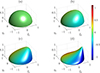Fig. 3 Degree of coherence for a sZegö source at the source plane relative to a point located at (a) ρ 2 = (0, 0); (b) ρ 2 = (0.3, 0); (c) ρ 2 = (0.6, 0); and (d) ρ 2 = (0.9, 0). Absolute value is represented on the vertical axis, and the phase is coded in a color scale.

The OAM degree of coherence at z = 0 can be derived using infinite geometric series. Together with the degree of orbitalization they take forms:$$o_S({\rho }_1,{\rho }_2,0)=\sqrt{\frac{(1-{\rho }_1^2)(1-{\rho }_2^2)}{1-{\rho }_1^2{\rho }_2^2}};O_S(\rho ,0)={\left(1-{\rho }^2\right)}^2.$$(33)

Note that O_S (ρ, 0) has a particularly simple form since for this source λ_n (ρ, 0) ≥ λ_n + 1(ρ, 0) for all n and ρ, which is not generally true for other source classes. The color density plot of the OAM degree of coherence for this beam is shown in Figure 4a. As expected, this quantity takes the unity value at ρ₁ = ρ₂ = 0 but gradually decreases and reaches zero for ρ₁ = 1 or ρ₂ = 1. We also note that it is not generally unity at the coinciding radii ρ₁ = ρ₂ ≠ 0, unlike the classic degree of coherence that would be at the coinciding points.

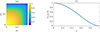Fig. 4 (a) OAM degree of coherence oS (ρ1, ρ2) and (b) degree of orbitalization OS (ρ) for a sZegö source.

An explicit expression of the CSD of the field radiated in the far zone, W_S,∞, can hardly be derived directly from the CSD in z = 0, but from its modal expansion, with the modes of equation (26) and the eigenvalues given by$${\lambda }_n=I_0\frac{\pi r_0^2}{n+1},\hspace{1em}(n=\mathrm{0,1},...),$$(34)takes the form$$W_{S,\infty }({\mathit{\nu }}_1,{\mathit{\nu }}_2)\propto \sum _{n=0}^{\infty }\mathrm{}\frac{J_{n+1}\left(2\pi r_0{\nu }_1\right)}{2\pi r_0{\nu }_1}\frac{J_{n+1}\left(2\pi r_0{\nu }_2\right)}{2\pi r_0{\nu }_2}{e}^{\mathrm{in}({\vartheta }_1-{\vartheta }_2)},$$(35)which can be used to evaluate S_S,∞ and μ_S,∞ numerically. The latter quantities, evaluated by adding the contribution of the first 100 modes, are shown in Figures 5 and 6, respectively.

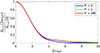Fig. 5 Spectral density for a sZegö source in the far field (with r0 = 1), calculated by adding the first 2, 5, and 100 modes, repectively.

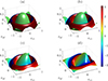Fig. 6 Degree of coherence for a sZegö source across a plane in the far zone relative to a point located at (a) v 2 = (0, 0); (b) v 2 = (0.16, 0); (c) v 2 = (0.32, 0); and (d) v 2 = (0.48, 0). Absolute value is represented on the vertical axis, and the phase is coded in a color scale. The first 100 modes were considered in the calculation.

For the case of the spectral density, it was found that there are no significant differences, at least in the range r₀ ν < 1, when calculating it using only the first 6 modes or the first 100 modes, so that the contribution of modes of order higher than 6 turns out to be negligible. Basically, the same conclusions hold for the degree of coherence, but in such a case, the first 10 modes have to be considered. The degree of coherence shows cylindrical symmetry when calculated in relation to the beam axis, with its absolute value reaching a maximum at the center of the beam and showing decreasing oscillations, while the phase alternates between 0 and π. When evaluated in relation to a direction outside the axis, the oscillations of the absolute value of the DOC are distorted, and the phase varies gradually. In this case also the presence of coherence vortices can be observed (with charge +1 and −1), corresponding to the zeros of μ_S,∞ [38]. The absolute value is represented on the vertical axis, and the phase is coded in a color scale. The first 100 modes were considered in the calculation.

The far-zone OAM degree of coherence of a field radiated by a sZegö source takes form$$o_S({\nu }_1,{\nu }_2)=\frac{2\sqrt{\sum _{n=0}^{\infty }\mathrm{}{J}_{n+1}^2\left(2\pi r_0{\nu }_1\right)J_{n+1}^2\left(2\pi r_0{\nu }_2\right)}}{\sqrt{1-J_0^2\left(2\pi r_0{\nu }_1\right)}\sqrt{1-J_0^2\left(2\pi r_0{\nu }_2\right)}},$$(36)after using a summation formula for $J_{n+1}^2\left(2\pi r_0{\nu }_j\right)$, j = 1, 2 in the denominator. Figure 7a shows this quantity as a function of ν₁, ν₂ with r₀ = 1, where we restrict ourselves to a region close to the axis. This distribution is structurally different from that in Figure 4a, since the coherence no longer decreases monotonically with the increasing radii but oscillates between wider and narrower distributions. It should also be noted that for ν₁ = ν₂ = ν the OAM coherence remains fairly high within the plotted region around the axis.

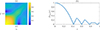Fig. 7 (a) OAM degree of coherence oS (ν1, ν2); (b) degree of orbitalization OS (ν) for a far field radiated by sZegö source.

The degree of orbitalization becomes$$O_S\left(\nu \right)=2\frac{J_p^2\left(2\pi r_0\nu \right)-J_q^2\left(2\pi r_0\nu \right)}{1-J_0^2\left(2\pi r_0\nu \right)},$$(37)where p and q are the indices of the largest and the second largest eigenvalues σ_n for a given radius ν. We note that unlike in the source plane, where the zeroth and the first eigenvalues are the largest and second largest for all radii, in the far field such eigenvalues must be determined numerically. Figure 7b shows the degree of orbitalization as a function of ν, with r₀ = 1, for ν ≤ 1. Unlike in the source plane, where this degree monotonically decreases from unity to zero, see Figure 4b, it shows a piecewise-continuous profile without smoothness at junctions. This is due to the fact that many OAM modes are competing for being the maximum and the second maximum. For example, close to the axis, modes n = 0 and n = 1 constitute this pair, but at ν ≈ 0.419, modes n = 1 and n = 2 become such. Hence, most of the oscillations are due to switching to higher indexes, with one exception: in the region 0.817 ≤ ν ≤ 0.894, the n = 0 mode has a crest becoming the second largest eigenvalue again.

4.2 Truncated sZegö sources

In this case, we let c_n  = I₀ if 0 ≤ n < N and c_n  = 0 if n ≥ N, so that equation (1) gives$$g_T\left(\zeta \right)=I_0\sum _{n=0}^{N-1}\mathrm{}{\zeta }^n=I_0\frac{1-{\zeta }^N}{1-\zeta }\hspace{1em}\left(\right|\zeta |<1),$$(38)and the corresponding CDS turns out to be$$W_T({\mathit{\rho }}_1,{\mathit{\rho }}_2,0)=I_0\frac{1-({\rho }_1{\rho }_2{)}^N{e}^{\mathrm{iN}({\phi }_1-{\phi }_2)}}{1-{\rho }_1{\rho }_2{e}^{i({\phi }_1-{\phi }_2)}};\hspace{1em}(0\le {\rho }_1,{\rho }_2<1).$$(39)

Spectral density and degree of coherence across the source plane turn out to be, from equations (15) and (16),$$S_T(\mathit{\rho },0)=I_0\frac{1-{\rho }^{2N}}{1-{\rho }^2}\mathrm{circ}\left(\rho \right),$$(40)and$${\mu }_T\left({\mathit{\rho }}_1,{\mathit{\rho }}_2,0\right)=\sqrt{\frac{\left(1-{\rho }_1^2\right)\left(1-{\rho }_2^2\right)}{\left(1-{\rho }_1^{2N}\right)\left(1-{\rho }_2^{2N}\right)}}\frac{1-({\rho }_1{\rho }_2{)}^N{e}^{\mathrm{iN}\left({\phi }_1-{\phi }_2\right)}}{1-{\rho }_1{\rho }_2{e}^{i\left({\phi }_1-{\phi }_2\right)}}\mathrm{circ}\left({\rho }_1\right)\mathrm{ }\mathrm{circ}\left({\rho }_2\right),$$(41)respectively. The plots of S_T and μ_T are shown in Figures 8 and 9, respectively. It can be seen that, as the number of modes increases, the spectral density becomes more and more similar to that of the sZegö source but never diverges, as expected. On the other hand, the DOC is highly dependent on the number of modes considered.

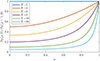Fig. 8 Spectral density at the source (normalized to the maximum) for a truncated sZegö CSD with N = 1, 2, 3, 5, 10, 20.

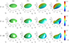Fig. 9 Degree of coherence at the source plane, for a truncated sZegö CSD with N = 2, 4, 20 (from top to bottom), relative to a point located at (a) ρ 2 = (0, 0); (b) ρ 2 = (0.3, 0); (c) ρ 2 = (0.6, 0); and (d) ρ 2 = (0.9, 0). Absolute value is represented on the vertical axis, and the phase is coded in a color scale.

Two aspects deserve to be noticed. First, the coherence area decreases as N increases, as expected. The second aspect concerns the phase structure of μ_T . It can be highlighted in a simpler way if we focus our attention on the second fraction in equation (41), provided the other terms are positive. Using again the variable ζ = ρ₁ ρ₂ exp[i(φ₁ − φ₂)], this term can be written as$$\frac{1-{\zeta }^N}{1-\zeta }=-\frac{\prod _{n=1}^N\mathrm{}(\zeta -{\zeta }_n)}{1-\zeta },$$(42)where ζ_n (n = 1, …, N) are the solutions of the equation ζ ^N = 1, namely, ζ_n = exp(i2πn/N). Therefore, since ζ_N = 1, we have$$-\frac{\prod _{n=1}^N\mathrm{}(\zeta -{\zeta }_n)}{1-\zeta }=\prod _{n=1}^{N-1}\mathrm{}(\zeta -{\zeta }_n),$$(43)which for fixed values of ρ₂ and φ₂ can be written as$$\prod _{n=1}^{N-1}\mathrm{}(\zeta -{\zeta }_n)={\rho }_2^{(N-1)}{e}^{-i(N-1){\phi }_2}\prod _{n=1}^{N-1}\mathrm{}\left[{\rho }_1{e}^{i{\phi }_1}-\frac{1}{{\rho }_2}{e}^{i({\phi }_2+2\pi n/N)}\right],$$(44)representing the product of N − 1 vortices, each having charge +1, centered on N − 1 vertices of a regular enneagon, at a distance 1/ρ₂ from the center.

To better understand this point, let us take φ₂ = 0. Then, the nth term of the product takes the form$${\rho }_1{e}^{i{\phi }_1}-\frac{1}{{\rho }_2}{e}^{i2\pi n/N}=\left[{\xi }_1-\frac{1}{{\rho }_2}\cos \left(\frac{2\pi n}{N}\right)\right]+i\left[{\eta }_1-\frac{1}{{\rho }_2}\sin \left(\frac{2\pi n}{N}\right)\right],$$(45)which actually represents a vortex with charge +1 and center at$${\mathit{\rho }}_1^{\left(n\right)}=\left(\frac{1}{{\rho }_2}\cos \left(\frac{2\pi n}{N}\right),\frac{1}{{\rho }_2}\sin \left(\frac{2\pi n}{N}\right)\right).$$(46)

The phase structure of the DOC is shown in Figure 10 for ρ ₂ = (0.9, 0) and several values of N.

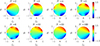Fig. 10 Phase of the degree of coherence at the source plane, for a truncated sZegö CSD relative to the point ρ 2 = (0.9, 0) for several values of N.

The OAM degree of coherence for this source at z = 0 can be derived using finite geometric series. This quantity and the degree of orbitalization take form$$o_T({\rho }_1,{\rho }_2,0)=\sqrt{\frac{(1-{\rho }_1^2)(1-{\rho }_2^2)}{1-{\rho }_1^2{\rho }_2^2}}\sqrt{\frac{1-{\rho }_1^{2N}{\rho }_2^{2N}}{(1-{\rho }_1^{2N})(1-{\rho }_2^{2N})}};{\hspace{1em}O}_T(\rho ,0)=\frac{(1-{\rho }^2{)}^2}{1-{\rho }^{2N}}.$$(47)

The plots of the OAM degree of coherence for this source are shown in Figures 11a–11c, for several values of N. Unlike for the sZegö sources the distributions do not decrease to zero for ρ₁ = 1 or ρ₂ = 1 but rather take on values in the interval (0, 1) decreasing with increasing N. The plots of the degree of orbitalization are shown in Figure 12 for several values of N. The case N = ∞ is also shown corresponding to the un-truncated sZegö source. While all the curves have monotonic behavior taking on unit value at ρ = 0 and decreasing to zero at ρ = 1 only the curve for N = 1 is convex on the whole interval, all the others change convexity once.

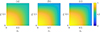Fig. 11 OAM degree of coherence oT (ρ1, ρ2) for truncated sZegö sources with (a) N = 4; (b) N = 8; (c) N = 16.

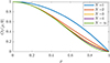Fig. 12 Degree of orbitalization OT (ρ) for truncated sZegö sources with different values of N. The case N = ∞ corresponds to the non-truncated sZegö source.

To evaluate the propagated CSD in the near and in the far field equations (14) and (19), or (26) are used. Equations (38) and (8) give, for the eigenvalues,$${\lambda }_n=\{\begin{array}{ll}{I}_0\frac{\pi r_0^2}{n+1}& (0\le n<N);\\ & \\ 0& (n\ge N).\end{array}$$(48)

Figure 13 shows examples of the spectral density, across the (x, z) plane, of the field propagated from sZegö sources of various orders. It can be observed that the main contribution for large propagation distances is due to the 0th order mode (compare Fig. 13 with Fig. 1 for n = 0).

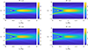Fig. 13 Spectral density versus the inverse of the Fresnel number for several truncated sZegö sources with N modes.

As commented above, the addition of more and more modes modifies the distribution of the spectral density only for small propagation distances. This is confirmed by the plots in Figure 14 where the spectral density profiles are calculated at several propagation distances for sZegö truncated sources with different numbers of modes. For a Fresnel number N_F = 4, the five profiles are different, although those corresponding to N = 30 and N = 100 are practically the same up to a normalized distance ρ = 1. For N_F = 1 the profiles practically coincide for all truncated sZegö sources with N ≥ 12. This profile should be the same as the one for sZegö source.

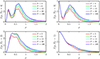Fig. 14 Spectral density versus the inverse of the Fresnel number for different truncated sZegö sources.

The same approach can be used to evaluate the degree of coherence across different planes (Fig. 15). The analogous calculations across the source plane and in the far field [38] showed the presence of coherence vortices (in both cases).

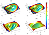Fig. 15 Degree of coherence relative to a point located at ρ 2 = (0, 0.5) for a truncated sZegö source with N = 4 at several propagation distances (a) NF  = 3; (b) NF  = 2; (c) NF  = 1; (d) NF  = 0.5. The absolute value is represented on the vertical axis, and the phase is coded in a color scale.

The far-zone OAM degree of coherence radiated by a truncated sZegö source takes the form$$o_T({\nu }_1,{\nu }_2)=\frac{\sqrt{\sum _{n=0}^{N-1}\mathrm{}{J}_{n+1}^2\left(2\pi r_0{v}_1\right)J_{n+1}^2\left(2\pi r_0{v}_2\right)}}{\prod _{j=\mathrm{1,2}}\mathrm{}\sqrt{\sum _{n=0}^{N-1}\mathrm{}{J}_{n+1}^2\left(2\pi r_0{v}_j\right)}}.$$(49)

Figure 16 shows this quantity for several values of the summation index: (a) N = 2, (b) N = 3, and (c) N = 4. As N increases, the distributions start resembling that for the non-truncated model, if compared to Figure 7a. This practically occurs already for N = 4, as higher-order modes deliver much smaller contributions to the sums.

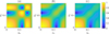Fig. 16 OAM degree of coherence oT (ν1, ν2) for truncated sZegö far fields with (a) N = 2; (b) N = 3; (c) N = 4.

For truncated sZegö far fields the degree of orbitalization becomes$$O_T\left(\nu \right)=\frac{J_p^2\left(2\pi r_0\nu \right)-J_q^2\left(2\pi r_0\nu \right)}{\sum _{n=0}^{N-1}\mathrm{}{J}_{n+1}^2\left(2\pi r_0\nu \right)},$$(50)where, as above, p and q are the indices of the largest and the second largest eigenvalues. Analogously to the non-truncated model, the determination of the largest and the second largest eigenvalues for different radii was carried out numerically.

Figure 17 shows formation of the degree of orbitalization for (a) N = 2 and (b) N = 3. For N = 2 the degree exhibits strictly oscillatory nature with smooth maxima and non-smooth minima, all at zeroes. This is due to the fact that only two modes compete with each other for being maximum and second maximum and can only alternate. This behavior is similar to that of the degree of polarization, also involving competition of two electric field components. Starting from N = 3 both maxima and minima are not smooth, since the switches are determined by three pairs of modes. Figure 17c summarizes the behavior for cases N = 2, N = 3 and N → ∞ (non-truncated model), same as in Figure 7b. In parts where the curves are almost the same, the same modes act as the largest and second largest eigenvalues resulting in the same numerator in equation (17), while the denominator has an increasing value with increasing N. This always occurs at small ν as the 0th mode always dominates close to the axis.

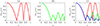Fig. 17 Degree of orbitalization OT (ν) for truncated sZegö far fields with (a) N = 2; (b) N = 3; (c) combination of N = 2, N = 3, and non-truncated model.

5 Further examples of uni-variable sources

Different uni-variable CSDs can be defined by choosing different sets of c_n coefficients, and in many cases they are given in closed form, as happened for the case in the previous section. Actually, using handbooks of mathematical formulas, dozens of other CSDs can be defined from formulas involving power series. Some of them lead to closed forms even when the series is truncated. This is particularly useful because, as we saw for sZegö and truncated sZegö sources, in such a case the effects of truncation can be evaluated quite simply. Furthermore, in any practical realization of partially coherent sources based on the superimposition of perfectly coherent and mutually uncorrelated fields, the number of modes must be necessarily truncated.

Among others, we quote the following (formula 5.2.2.4 of [64]):$$g\left(\zeta \right)=I_0\sum _{n=1}^{\infty }\mathrm{}n{\zeta }^n=I_0 \frac{\zeta }{(1-\zeta {)}^2},$$(51)together with its truncated version (formula 4.1.7.2 of [64])$$g_T\left(\zeta \right)=I_0\sum _{n=1}^N\mathrm{}n{\zeta }^n=I_0\frac{\zeta +(\mathrm{N\zeta }-N-1) {\zeta }^{N+1}}{(1-\zeta {)}^2},$$(52)with integer N.

Another interesting example of a source obtained with a finite number of modes is that of the binomial source, for which (formula 4.2.3.1 of [64])$$g\left(\zeta \right)=I_0\sum _{n=0}^N\mathrm{}\left(\begin{array}{l}N\\ n\end{array}\right){\zeta }^n=I_0(1+\zeta {)}^N.$$(53)

As a last example, we quote the following, which will be discussed in a little more detail. If we take (formula 5.2.7.2 of [64])$$g\left(\zeta \right)=I_0\sum _{n=0}^{\infty }\mathrm{}\frac{{\left({\gamma }^2\zeta \right)}^n}{n!}=I_0{e}^{{\gamma }^2\zeta },$$(54)with γ ² a positive dimensionless parameter, the corresponding uni-variable CSD turns out to be$$W_G({\mathit{\rho }}_1,{\mathit{\rho }}_2)=I_0\exp \left\{{\gamma }^2{\rho }_1{\rho }_2\exp \left[i({\phi }_1-{\phi }_2)\right]\right\}\mathrm{circ}\left({\rho }_1\right)\mathrm{circ}\left({\rho }_2\right),$$(55)and the corresponding spectral density has the form$$S_G\left(\rho \right)=I_0{e}^{{\gamma }^2{\rho }^2}\mathrm{circ}\left(\rho \right).$$(56)

The interest in such sources comes from what follows. If we express W_G through the vectors ρ ₁ and ρ ₂, since ρ _j = (ξ_j , η_j ) and ρ_j exp(iφ_j ) = ξ_j  + iη_j , (j = 1, 2), equation (55) can also be written as$$\begin{array}{c}{W_G\left({\mathit{\rho }}_1,{\mathit{\rho }}_2\right)=I}_0{e}^{{\gamma }^2({\xi }_1{\xi }_2+{\eta }_1{\eta }_2)}{e}^{-i{\gamma }^2({\xi }_1{\eta }_2-{\xi }_2{\eta }_1)}\mathrm{circ}\left({\rho }_1\right)\mathrm{circ}\left({\rho }_2\right)\\ =I_0{e}^{{\gamma }^2 {\mathit{\rho }}_1\cdot {\mathit{\rho }}_2} e^{-i{\gamma }^2({\mathit{\rho }}_1\times {\mathit{\rho }}_2{)}_z} \mathrm{circ}\left({\rho }_1\right)\mathrm{circ}\left({\rho }_2\right)\end{array}$$(57)or, after some manipulations,$$W_G({\mathit{\rho }}_1,{\mathit{\rho }}_2)=I_0{e}^{{\gamma }^2({\rho }_1^2+{\rho }_2^2)/2}{e}^{-{\gamma }^2{\left|{\mathit{\rho }}_1-{\mathit{\rho }}_2\right|}^2/2}{e}^{-i{\gamma }^2({\mathit{\rho }}_1\times {\mathit{\rho }}_2{)}_z}\mathrm{circ}\left({\rho }_1\right)\mathrm{circ}\left({\rho }_2\right),$$(58)which apparently has the form of a twisted Gaussian Schell-model source with saturated twist [40], the only difference being the sign in the argument of the Gaussian amplitude term. In particular, the degree of coherence turns out to be$${\mu }_G({\mathit{\rho }}_1,{\mathit{\rho }}_2)=e^{-{\gamma }^2{\left|{\mathit{\rho }}_1-{\mathit{\rho }}_2\right|}^2/2}{e}^{-i{\gamma }^2({\mathit{\rho }}_1\times {\mathit{\rho }}_2{)}_z}\mathrm{circ}\left({\rho }_1\right)\mathrm{circ}\left({\rho }_2\right),$$(59)whose modulus is$$\left|{\mu }_G({\mathit{\rho }}_1,{\mathit{\rho }}_2)\right|=e^{-{\gamma }^2{\left|{\mathit{\rho }}_1-{\mathit{\rho }}_2\right|}^2/2}\mathrm{circ}\left({\rho }_1\right)\mathrm{circ}\left({\rho }_2\right).$$(60)

The eigenvalues of the Mercer expansion of W_G turn out to be$${\lambda }_n=I_0{\gamma }^{2n}\frac{\pi r_0^2}{(n+1)!},$$(61)from which the propagation features of the radiated beams could be evaluated.

In this case, too, the truncated version of the series can be expressed in closed form because (formula 4.1.7.10 of [64])$$g_T\left(\zeta \right)=I_0\sum _{n=0}^N\mathrm{}\frac{{\left({\gamma }^2\zeta \right)}^n}{n!}=I_0\frac{\mathrm{\Gamma }\left(N+1,{\gamma }^2\zeta \right)}{N!}{e}^{{\gamma }^2\zeta },$$(62)where Γ(·,·) is the incomplete Gamma function [63].

6 Conclusions

Uni-variable CSDs can be derived from any function of a single complex argument whose Taylor series involves only non-negative coefficients. The convergence range of the series determines the spatial extent of the source. The Taylor series can be directly related to the Mercer expansion of the CSD of the source in such a way that the coherent modes turn out to be optical vortices, restricted to a circle at the source plane, and the corresponding eigenvalues are proportional to the Taylor coefficients.

Although the coherence features of light across the source plane can be directly derived from the analytical form of the CSD, the analogous properties for the radiated beam can hardly be evaluated in closed form. Nevertheless, from the knowledge of modes and eigenvalues of the CSD across the source, the coherence features of the radiated beam can be evaluated both in the Fresnel regime and in the Fraunhofer regime.

In this paper, the tools for studying the properties of the propagated field have been provided and applied to a test case, that is, the sZegö source. Furthermore, the effects, on the coherence properties of the source and the radiated field, of truncating the Taylor series have also been investigated. This is crucial from an experimental point of view, because limiting the Taylor series (i.e., the coherent-mode expansion of the CSD) to a finite number of terms becomes necessary whenever sources of this kind have to be synthesized through the superposition of mutually uncorrelated perfectly coherent fields.

Since the coherent modes of uni-variable CSDs possess vortex-like structures at various OAM indices, the overall fields can be regarded as carrying OAM in multiple states. Hence, besides the spectral density and the degree of coherence, which carry information about correlations in the physical space, some recently introduced measures, namely, the OAM degree of coherence and the degree of orbitalization, have also been invoked to characterize the radial correlations of the investigated sources in the OAM space, i.e., the polar Fourier space. Although the technique presented here has been applied to the sZegö CSD and to its truncated version (the truncated sZegö CSD), it can be applied to any source of the uni-variable type. The number of uni-variable CSD that can be envisaged starting from the Taylor expansion of a single-argument function is actually huge, and this work lays the foundation for the design and tayloring of sources with required coherence characteristics, both on the source plane and in propagation.

Funding

This work has been supported by the Spanish Ministerio de Economía y Competitividad under project PID2023-148021NB-I00 and Project FASLIGTH (RED2022-134391-T).

Conflicts of interest

This work has no financial or non-financial competing interests.

Data availability statement

Data will be made available on request.

Author contribution statement

All authors have contributed equally to all aspects of this work, including conceptualization, methodology, formal analysis, and the writing of the original draft and final manuscript.

References

All Figures

	Fig. 1 Density plots of the spectral density of some modes, |Φn ( r , z)|2, across the plane (ξ, z) for n = 0, 1, 2, 3, 4, 5.
In the text

	Fig. 2 Plots of the spectral density of the modes in the far field, equation (26) for n = 5 (a), 10 (b), 15 (c), with r0 = 1.
In the text

	Fig. 3 Degree of coherence for a sZegö source at the source plane relative to a point located at (a) ρ 2 = (0, 0); (b) ρ 2 = (0.3, 0); (c) ρ 2 = (0.6, 0); and (d) ρ 2 = (0.9, 0). Absolute value is represented on the vertical axis, and the phase is coded in a color scale.
In the text

	Fig. 4 (a) OAM degree of coherence oS (ρ1, ρ2) and (b) degree of orbitalization OS (ρ) for a sZegö source.
In the text

	Fig. 5 Spectral density for a sZegö source in the far field (with r0 = 1), calculated by adding the first 2, 5, and 100 modes, repectively.
In the text

	Fig. 6 Degree of coherence for a sZegö source across a plane in the far zone relative to a point located at (a) v 2 = (0, 0); (b) v 2 = (0.16, 0); (c) v 2 = (0.32, 0); and (d) v 2 = (0.48, 0). Absolute value is represented on the vertical axis, and the phase is coded in a color scale. The first 100 modes were considered in the calculation.
In the text

	Fig. 7 (a) OAM degree of coherence oS (ν1, ν2); (b) degree of orbitalization OS (ν) for a far field radiated by sZegö source.
In the text

	Fig. 8 Spectral density at the source (normalized to the maximum) for a truncated sZegö CSD with N = 1, 2, 3, 5, 10, 20.
In the text

	Fig. 9 Degree of coherence at the source plane, for a truncated sZegö CSD with N = 2, 4, 20 (from top to bottom), relative to a point located at (a) ρ 2 = (0, 0); (b) ρ 2 = (0.3, 0); (c) ρ 2 = (0.6, 0); and (d) ρ 2 = (0.9, 0). Absolute value is represented on the vertical axis, and the phase is coded in a color scale.
In the text

	Fig. 10 Phase of the degree of coherence at the source plane, for a truncated sZegö CSD relative to the point ρ 2 = (0.9, 0) for several values of N.
In the text

	Fig. 11 OAM degree of coherence oT (ρ1, ρ2) for truncated sZegö sources with (a) N = 4; (b) N = 8; (c) N = 16.
In the text

	Fig. 12 Degree of orbitalization OT (ρ) for truncated sZegö sources with different values of N. The case N = ∞ corresponds to the non-truncated sZegö source.
In the text

	Fig. 13 Spectral density versus the inverse of the Fresnel number for several truncated sZegö sources with N modes.
In the text

	Fig. 14 Spectral density versus the inverse of the Fresnel number for different truncated sZegö sources.
In the text

	Fig. 15 Degree of coherence relative to a point located at ρ 2 = (0, 0.5) for a truncated sZegö source with N = 4 at several propagation distances (a) NF  = 3; (b) NF  = 2; (c) NF  = 1; (d) NF  = 0.5. The absolute value is represented on the vertical axis, and the phase is coded in a color scale.
In the text

	Fig. 16 OAM degree of coherence oT (ν1, ν2) for truncated sZegö far fields with (a) N = 2; (b) N = 3; (c) N = 4.
In the text

	Fig. 17 Degree of orbitalization OT (ν) for truncated sZegö far fields with (a) N = 2; (b) N = 3; (c) combination of N = 2, N = 3, and non-truncated model.
In the text

References

- Yu J, Zhu X, Wang F, Chen Y, Cai Y, Research progress on manipulating spatial coherence structure of light beam and its applications, Prog. Quantum Electron. 91–92, 100486 (2023). https://doi.org/10.1016/j.pquantelec.2023.100486. [Google Scholar]
- Rosales-Guzmán C, Rodríguez-Fajardo V, A perspective on structured light’s applications, Appl. Phys. Lett. 125, 200503 (2024). https://doi.org/10.1063/5.0236477. [Google Scholar]
- Liang C, Wu G, Wang F, Li W, Cai Y, Ponomarenko SA, Overcoming the classical Rayleigh diffraction limit by controlling two-point correlations of partially coherent light sources, Opt. Express 25, 28352 (2017). https://doi.org/10.1364/OE.25.028352. [Google Scholar]
- Shen Y, Sun H, Peng D, Chen Y, Cai Q, Wu D, Wang F, Cai Y, Ponomarenko SA, Optical image reconstruction in 4f imaging system: Role of spatial coherence structure engineering, Appl. Phys. Lett. 118, 181102 (2021). https://doi.org/10.1063/5.0046288. [Google Scholar]
- Gibson G, Courtial J, Padgett MJ, Vasnetsov M, Pas’ko V, Barnett SM, Franke-Arnold S, Free-space information transfer using light beams carrying orbital angular momentum, Opt. Express 12, 5448 (2004). https://doi.org/10.1364/OPEX.12.005448. [CrossRef] [Google Scholar]
- Wang J, et al., Terabit free-space data transmission employing orbital angular momentum multiplexing, Nat. Photonics 6, 488 (2012). https://doi.org/10.1038/nphoton.2012.138. [NASA ADS] [CrossRef] [Google Scholar]
- Liu X, Shen Y, Liu L, Wang F, Cai Y, Experimental demonstration of vortex phase-induced reduction in scintillation of a partially coherent beam, Opt. Lett. 38, 5323 (2013). https://doi.org/10.1364/OL.38.005323. [Google Scholar]
- Gbur G, Partially coherent beam propagation in atmospheric turbulence, J. Opt. Soc. Am. A 31, 2038 (2014). https://doi.org/10.1364/JOSAA.31.002038. [Google Scholar]
- Lin S, Zhu X, Shen Y, Wang F, Chen X, Gbur G, Cai Y, Yu J, Statistically stationary random light for high-security encryption, Optica 12, 1261 (2025). https://doi.org/10.1364/OPTICA.546899. [Google Scholar]
- Zhao C, Cai Y, Trapping two types of particles using a focused partially coherent elegant Laguerre–Gaussian beam, Opt. Lett. 36, 2251 (2011). https://doi.org/10.1364/OL.36.002251. [Google Scholar]
- Zhang Z, Liu X, Wang H, Liang C, Cai Y, Zeng J, Flexible optical trapping and manipulating Rayleigh particles via the cross-phase modulated partially coherent vortex beams, Opt. Express 32, 35051 (2024). https://doi.org/10.1364/OE.539069. [Google Scholar]
- Guo J, Ming S, Wu Y, Chen LQ, Zhang W, Super-sensitive rotation measurement with an orbital angular momentum atom-light hybrid interferometer, Opt. Express 29, 208 (2021). https://doi.org/10.1364/OE.409964. [Google Scholar]
- Gori F, Santarsiero M, Devising genuine spatial correlation functions, Opt. Lett. 32, 3531 (2007). https://doi.org/10.1364/OL.32.003531. [Google Scholar]
- Martínez-Herrero R, Mejías PM, Gori F, Genuine cross-spectral densities and pseudo-modal expansions, Opt. Lett. 34, 1399 (2009). https://doi.org/10.1364/OL.34.001399. [Google Scholar]
- Raghunathan SB, van Dijk T, Peterman EJG, Visser TD, Experimental demonstration of an intensity minimum at the focus of a laser beam created by spatial coherence: application to the optical trapping of dielectric particles, Opt. Lett. 35, 4166 (2010). https://doi.org/10.1364/OL.35.004166. [Google Scholar]
- Gbur G, Visser TD, The structure of partially coherent fields, Prog. Opt. 55, 285 (2010). https://doi.org/10.1016/B978-0-444-53705-8.00005-9. [Google Scholar]
- Wu G, Cai Y, Detection of a semirough target in turbulent atmosphere by a partially coherent beam, Opt. Lett. 36, 1939 (2011). https://doi.org/10.1364/OL.36.001939. [Google Scholar]
- Lajunen H, Saastamoinen T, Propagation characteristics of partially coherent beams with spatially varying correlations, Opt. Lett. 36, 4104 (2011). https://doi.org/10.1364/OL.36.004104. [Google Scholar]
- Cai Y, Chen Y, Wang F, Generation and propagation of partially coherent beams with nonconventional correlation functions: a review, J. Opt. Soc. Am. A 31, 2083 (2014). https://doi.org/10.1364/JOSAA.31.002083. [Google Scholar]
- Rodenburg B, Mirhosseini M, Magaña-Loaiza OS, Boyd RW, Experimental generation of an optical field with arbitrary spatial coherence properties, J. Opt. Soc. Am. B 31, A51 (2014). https://doi.org/10.1364/JOSAB.31.000A51. [Google Scholar]
- Divitt S, Novotny L, Spatial coherence of sunlight and its implications for light management in photovoltaics, Optica 2, 95 (2015). https://doi.org/10.1364/OPTICA.2.000095. [Google Scholar]
- Chen Y, Ponomarenko SA, Cai Y, Experimental generation of optical coherence lattices, Appl. Phys. Lett. 109, 061107 (2016). https://doi.org/10.1063/1.4960966. [Google Scholar]
- Hyde MW IV, Bose-Pillai SR, Wood RA, Synthesis of non-uniformly correlated partially coherent sources using a deformable mirror, Appl. Phys. Lett. 111, 101106 (2017). https://doi.org/10.1063/1.4994669. [Google Scholar]
- Santarsiero M, Martínez-Herrero R, Maluenda D, de Sande JCG, Piquero G, Gori F, Partially coherent sources with circular coherence, Opt. Lett. 42, 1512 (2017). https://doi.org/10.1364/OL.42.001512. [Google Scholar]
- Santarsiero M, Martínez-Herrero R, Maluenda D, de Sande JCG, Piquero G, Gori F, Synthesis of circularly coherent sources, Opt. Lett. 42, 4115 (2017). https://doi.org/10.1364/OL.42.004115. [Google Scholar]
- Ding C, Koivurova M, Turunen J, Pan L, Self-focusing of a partially coherent beam with circular coherence, J. Opt. Soc. Am. A 34, 1441 (2017). https://doi.org/10.1364/JOSAA.34.001441. [Google Scholar]
- Piquero G, Santarsiero M, Martínez-Herrero R, de Sande JCG, Alonzo M, Gori F, Partially coherent sources with radial coherence, Opt. Lett. 43, 2376 (2018). https://doi.org/10.1364/OL.43.002376. [Google Scholar]
- Chen X, Li J, Rafsanjani SMH, Korotkova O, Synthesis of Im -Bessel correlated beams via coherent modes, Opt. Lett. 43, 3590 (2018). https://doi.org/10.1364/OL.43.003590. [Google Scholar]
- Wu D, Wang F, Cai Y, High-order nonuniformly correlated beams, Opt. Laser Technol. 99, 230 (2018). https://doi.org/10.1016/j.optlastec.2017.09.007. [Google Scholar]
- Martínez-Herrero R, Piquero G, de Sande JCG, Santarsiero M, Gori F, Besinc pseudo-Schell model sources with circular coherence, Appl. Sci. Basel 9, 2716 (2019). https://doi.org/10.3390/app9132716. [Google Scholar]
- de Sande JCG, Martínez-Herrero R, Piquero G, Santarsiero M, Gori F, Pseudo-Schell model sources, Opt. Express 27, 3963 (2019). https://doi.org/10.1364/OE.27.003963. [Google Scholar]
- Zhu X, Yu J, Chen Y, Wang F, Korotkova O, Cai Y, Experimental synthesis of random light sources with circular coherence by digital micro-mirror device, Appl. Phys. Lett. 117, 121102 (2020). https://doi.org/10.1063/5.0024283. [Google Scholar]
- Martínez-Herrero R, Santarsiero M, Piquero G, de Sande JCG, A new type of shape-invariant beams with structured coherence: Laguerre-Christoffel-Darboux beams, Photonics 8, 134 (2021). https://doi.org/10.3390/photonics8040134. [Google Scholar]
- Santarsiero M, Martínez-Herrero R, Piquero G, de Sande JCG, Gori F, Modal analysis of pseudo-Schell model sources, Photonics 8, 449 (2021). https://doi.org/10.3390/photonics8100449. [Google Scholar]
- Martínez-Herrero R, Piquero G, Santarsiero M, Gori F, de Sande JCG, A class of vectorial pseudo-Schell model sources with structured coherence and polarization, Opt. Laser Technol. 152, 108079 (2022). https://doi.org/10.1016/j.optlastec.2022.108079. [Google Scholar]
- Korotkova O, Gbur G, in A Tribute to Emil Wolf. Progress in Optics, Vol. 65, edited by T.D. Visser (Elsevier, 2020), pp. 43–104. [Google Scholar]
- Moreno-Acosta P, Rickenstorff-Parrao C, Ramirez-San-Juan JC, Rosales-Guzman C, Ramos-Garcia R, Experimental generation of partially coherent besinc pseudo-Schell model sources using a digital micromirror device, J. Opt. Soc. Am. B 42, 1804 (2025). https://doi.org/10.1364/JOSAB.564315. [Google Scholar]
- Gori F, Santarsiero M, Martínez-Herrero R, Uni-variable cross-spectral densities, Opt. Laser Technol. 180, 111511 (2025). https://doi.org/10.1016/j.optlastec.2024.111511. [Google Scholar]
- Indebetouw G, Optical vortices and their propagation, J. Mod. Opt. 40, 73 (1993). https://doi.org/10.1080/09500349314550101. [Google Scholar]
- Simon R, Mukunda N, Twisted Gaussian Schell-model beams, J. Opt. Soc. Am. A 10, 95 (1993). https://doi.org/10.1364/JOSAA.10.000095. [Google Scholar]
- Gori F, Santarsiero M, Borghi R, Vicalvi S, Partially coherent sources with helicoidal modes, J. Mod. Opt. 45, 539 (1998). https://doi.org/10.1080/09500349808231913. [Google Scholar]
- Ponomarenko SA, A class of partially coherent beams carrying optical vortices, J. Opt. Soc. Am. A 18, 150 (2001). https://doi.org/10.1364/JOSAA.18.000150. [Google Scholar]
- Gbur G, Visser TD, Coherence vortices in partially coherent beams, Opt. Commun. 222, 117 (2003). https://doi.org/10.1016/S0030-4018(03)01606-7. [Google Scholar]
- Tamburini F, Anzolin G, Umbriaco G, Bianchini A, Barbieri C, Overcoming the Rayleigh criterion limit with optical vortices, Phys. Rev. Lett. 97, 163903 (2006). https://doi.org/10.1103/PhysRevLett.97.163903. [Google Scholar]
- Franke-Arnold S, Allen L, Padgett M, Advances in optical angular momentum, Laser Photonics Rev. 2, 299 (2008). https://doi.org/10.1002/lpor.200810007. [NASA ADS] [CrossRef] [Google Scholar]
- Padgett M, Bowman R, Tweezers with a twist, Nat. Photonics 5, 343 (2011). https://doi.org/10.1038/nphoton.2011.81. [Google Scholar]
- Mirhosseini M, Magaña-Loaiza OS, Chen C, Rodenburg B, Malik M, Boyd RW, Rapid generation of light beams carrying orbital angular momentum, Opt. Express 21, 30196 (2013). https://doi.org/10.1364/OE.21.030196. [Google Scholar]
- Ambuj A, Vyas R, Singh S, Diffraction of orbital angular momentum carrying optical beams by a circular aperture, Opt. Lett. 39, 5475 (2014). https://doi.org/10.1364/OL.39.005475. [Google Scholar]
- Gbur G, Singular Optics, 1st edn. (CRC Press, 2016), ISBN 978-0521642224. [Google Scholar]
- Zeng J, Lin R, Liu X, Zhao C, Cai Y, Review on partially coherent vortex beams, Front. Optoelectron. 12, 229 (2019). https://doi.org/10.1007/s12200-019-0901-x. [Google Scholar]
- Zhang Y, Cai Y, Gbur G, Control of orbital angular momentum with partially coherent vortex beams, Opt. Lett. 44, 3617 (2019). https://doi.org/10.1364/OL.44.003617. [Google Scholar]
- Liu X, Zeng J, Cai Y, Review on vortex beams with low spatial coherence, Adv. Phys. X 4, 1626766 (2019). https://doi.org/10.1080/23746149.2019.1626766. [Google Scholar]
- Zhang H, Lu X, Wang Z, Konijnenberg AP, Wang H, Zhao C, Cai Y, Generation and propagation of partially coherent power-exponent-phase vortex beam, Front. Phys. 9, 781688 (2021). https://doi.org/10.3389/fphy.2021.781688. [Google Scholar]
- Hyde IV MW, Korotkova O, Spencer MF, Partially coherent sources whose coherent modes are spatiotemporal optical vortex beams, J. Opt. 25, 035606 (2023). https://doi.org/10.1088/2040-8986/acba2d. [Google Scholar]
- Mandel L, Wolf E, Optical Coherence and Quantum Optics (Cambridge University Press, 1995), ISBN 9780521417112. [Google Scholar]
- Siegman AE, Lasers (University Science Books, 1986), ISBN 0935702113. [Google Scholar]
- Korotkova O, Gbur G, Unified matrix representation for spin and orbital angular momentum in partially coherent beams, Phys. Rev. A 103, 023529 (2021). https://doi.org/10.1103/PhysRevA.103.023529. [Google Scholar]
- Korotkova O, Pokharel S, OAM degree of coherence, Opt. Lett. 49, 5103 (2024). https://doi.org/10.1364/OL.528291. [Google Scholar]
- Korotkova O, Orbitalization ellipse of a light beam, Opt. Lett. 50, 391 (2025). https://doi.org/10.1364/OL.545613. [Google Scholar]
- Korotkova O, Orbitalization structure of random light beams, J. Opt. 27, 065606 (2025). https://doi.org/10.1088/2040-8986/addc7c. [Google Scholar]
- Born M, Wolf E, Principles of Optics, 7th (corrected) edn. (Cambridge University Press, 1999), ISBN 978-0521642224. [Google Scholar]
- Gradshteiin IS, Ryzhik IM, Table of Integrals, Series, and Products, 4th edn. (Academic Press, 1965). [Google Scholar]
- Abramowitz M, Stegun I, eds., Handbook of mathematical functions (Dover Publications Inc, 1972). [Google Scholar]
- Prudnikov A, Brychkov Y, Marichev O, Integrals and Series, Vol. 1: Elementary Functions (Gordon and Breach Science Publisher, 1986). [Google Scholar]