© The Author(s), published by EDP Sciences, 2025

1 Introduction

Optical frequency comb (OFC) generation based on second-harmonic (SH) nonlinear frequency conversion was first demonstrated in a bow-tie optical cavity [1, 2], and a cascade of χ⁽²⁾ processes was found to mimic a Kerr effect resulting in a modulation-instability (MI) OFC regime [3]. Besides, Kerr whispering-gallery-mode resonators with a toroidal shape have been used to generate octave-spanning microcombs [4] and temporal cavity solitons (CSs) [5], as predicted a couple of decades earlier [6].

Today, novel architectures have been demonstrated to excite robust CSs dynamical attractors [7], while innovative pumping schemes, such as chirped-pulse pumping, have been proposed to achieve complete control on the CS dynamics [8]. In the same context, on-chip integration of quadratic platforms at the μm-size scale is receiving increasing attention with a view to possibly achieving lower-power pump thresholds [9]. This is witnessed by the recent records of χ⁽²⁾ microring optical parametric oscillator (OPO) [10], Pockels micro-comb [11], and bicolor CSs [12].

At the same time, III-V semiconductors have proven interesting for nonlinear optical applications due to their energy bandgap tunability, which provides direct solutions for waveguide-dispersion engineering, and their typically high second- and third-order nonlinear response. As such, they led to paradigmatic demonstrations: SH vortex generation [13] and spin-orbit coupling [14] using nonlinear metasurfaces, entangled-photon sources [15, 16], ultralow-power Kerr OFC [17, 18], and photonic crystal cavity (PhC) OPO [19, 20]. Moreover, second harmonic generation (SHG) has been reported for (Al)GaAs [21–23] and (In)GaP alloys in both type I [24, 25] and type II [16, 26, 27] phase-matching (PM) schemes. Further perspective examples are broadband SHG [28] and electrically injected OPO [29].

Here, to model the OFC generation in a SHG-Kerr cavity [30, 31], we consider a double-envelope mean-field model, as was previously done to describe e.g. the field evolution of SHG [32, 33] and third-harmonic generation (THG) [34] in doubly resonant cavities. With this approach, one can predict Kerr-induced MI [35] and bistable soliton solutions [36] in a waveguide configuration. The case of an OPO resonator was presented in reference [37], and a two-wave model was used to describe the interplay between χ⁽³⁾ and χ⁽²⁾ surface effects in a silicon-nitride resonator [38]. As a general rule, whenever a non-negligible frequency conversion occurs into far different spectral domains, multi-envelope mean-field models are more convenient [39].

The scheme of our OFC generation setup is shown in Figure 1a. A monochromatic continuous-wave (CW) driving field S, around a resonance frequency ν₀ = ω₀/2π, is coupled evanescently in a SHG-Kerr ring resonator from a bus waveguide. Thanks to quadratic nonlinear effects, an important fraction of power is converted to the SH at 2ω₀. The intracavity field consists of two nonlinearly coupled waves (A, B), whose spectral broadening is due to the χ⁽²⁾ + χ⁽³⁾ interactions. The resulting output OFC owns spectral components around both the carriers ω₀ and 2ω₀. Figure 1b provides our technological choice for the waveguide cross-section: an AlGaAs core on top of a SiO₂ cladding and a Si wafer.

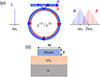Figure 1 (a) Scheme of a passively driven doubly resonant SHG-Kerr ring resonator. (b) Transverse cross-section with height h and width w.

In the following, we present the two-wave nonlinear dynamics resulting from the χ⁽²⁾ + χ⁽³⁾ interplay in AlGaAs waveguides. Since we focus on the relevant case of a pump wavelength in the telecom range, we discuss the crucial problem of the strong normal dispersion in the spectral domain around the SH λ_SH ∼ 0.775 μm. A valid solution is represented by a systematic dispersion engineering approach, which exploits local Bragg mirroring effects [40] and resonance frequency splittings [41] in a hybrid PhC-microring system [42]. Novel inverse design techniques of waveguides [43] or microcombs [44] address this specific topic.

The manuscript is organized as follows: in Section 2 we present the design of a doubly resonant AlGaAs microring; in Section 3 we model the resulting SHG-Kerr comb generation dynamics; in Section 4 we propose a purely χ⁽²⁾ optical feedback and we model the SHG; in Section 5 we discuss fabrication and present preliminary linear measurements; finally, in Section 6 we draw our conclusions and give some perspectives.

2 AlGaAs ring design

The alloy Al_0.18Ga_0.82As was chosen to both guarantee a high χ⁽²⁾ (${\chi }_{\mathrm{xyz}}^{\left(2\right)}\sim 238$ pm/V at λ ∼ 1.55 μm [45]) and avoid two-photon absorption (TPA) at λ₀ = 1.55 μm.

The AlGaAs crystal allows to achieve directional quasi phase matching ($\bar{4}$-QPM) between guided modes at ω₀ and 2ω₀ [46, 47], and the main design parameters are the waveguide width w, height h and bending radius R. Since optimal dispersion for Kerr-comb excitation around ω₀ occurs for waveguide cross sections with (h, w) ∼ (400, 600) nm [17, 18], we investigate geometries with h = 400 nm and we let w free to vary around its optimum.

2.1 Phase matching and frequency doubling efficiency

We make use of a commercial software (Lumerical, package FDE [48]) to compute the waveguide eigenmodes and their effective index (n_eff). A modal PM condition between fundamental transverse modes (either TE₀₀ or TM₀₀) at the driving wavelength and a higher-order transverse mode (TE₀₂) at SH is found. The energy density of the phase-matched eigenmodes is reported in Figure 2a, while Figure 2b reports the PM diagram of n_eff as a function of the waveguide width. The blue marker corresponds to a type-II PM point, found for w ∼ 470 nm. This occurs as the average of the n_eff of two pump modes (black dashed line) equals the n_eff of the SH mode. The red marker indicates a type-I PM point (found for w ∼ 610 nm), which occurs whenever the effective index of the pump mode is equal to that of the SH.

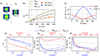Figure 2 (a) Energy density of the phase-matched guided modes at ω0 (TE00 and TM00) and 2ω0 (TE02,SH). (b) neff vs. w diagram of type-I (red marker) and type-II (blue marker) modal PM. (c) SHG efficiency as a function of the angle θ between the propagation direction and the [100] axis. (d) Effective index neff, (e) group velocity β1, and (f) GVD β2 for the TE00,FF (blue dashed line), TM00,FF (blue pointed line) and TE02,SH modes (red dashed line). In (d, e, f) the colored arrows indicate the corresponding x-axis.

We next compute the SHG efficiency [25, 26]:$$\kappa =\frac{{\omega }_0{ϵ}_0}{4}{\int }_{\mathrm{\Omega }}\mathrm{}{\chi }_{\mathrm{xyz}}^{\left(2\right)}{\mathbf{e}}_{2{\omega }_0}^{x,\mathrm{*}}\left({\mathbf{e}}_{{\omega }_0,1}^y{\mathbf{e}}_{{\omega }_0,2}^z+{\mathbf{e}}_{{\omega }_0,2}^y{\mathbf{e}}_{{\omega }_0,1}^z\right)\mathrm{d}\mathrm{\Omega },$$(1)where ${\mathbf{e}}_{{\omega }_0,1}$, ${\mathbf{e}}_{{\omega }_0,2}$ and ${\mathbf{e}}_{2{\omega }_0}$ are the electric fields at ω₀ and 2ω₀, respectively, Ω is the waveguide cross-section, χ⁽²⁾ is the second order susceptibility tensor, ϵ₀ is the electric permittivity, and x, y and z are the spatial coordinates. The symbol * indicates the complex conjugate, and tensor index contraction follows the Einstein summation convention. In equation (1) we use the standard normalization ${\mathbf{e}}_{\mathrm{norm}}=\mathbf{e}/\sqrt{N}$ [25], with $N=(1/2)\int (\mathbf{e}\times {\mathbf{h}}^{*})·\widehat{\mathbf{x}} \mathrm{d\Omega }, \mathbf{h}$ the magnetic field, $\widehat{\mathbf{x}}$ the propagation direction and × the vector product. Since ${\chi }_{\mathrm{xyz}}^{\left(2\right)}$ is a tensor, κ is strongly influenced by the orientation of the propagation direction with respect to the crystalline axes. For this reason we define θ as the angle, in the (001) plane, between the propagation direction and the [100] axis. The SHG generation efficiency |κ|² is reported in Figure 2c for both type-I and type-II PM conditions. We note that the κ assumes comparable values in these two cases. In what follows we will consider the type-I PM case for two main reasons: 1) it results in a better dispersion profile; 2) for the type-II modal PM we are close to a degeneracy point w = h, which is detrimental for broadband applications. Finally, as introduced above, in a ring configuration the condition $\bar{4}$-QPM implies slightly different optimal w. The corresponding waveguide cross-section is thus set as (w, h) = (630, 400) nm.

2.2 Chromatic dispersion

Chromatic dispersion plays a pivotal role for broadband frequency generation, as the propagation constant has a different spectral dependence for each mode. It is convenient to expand it in Taylor series around a carrier frequency ω₀ [49]:$$\beta \left(\omega \right)=n_{\mathrm{eff}}\left(\omega \right)\frac{\omega }{c}=\sum _k\mathrm{}{\beta }_k\frac{[\omega -{\omega }_0{]}^k}{k!},$$(2)where ${\beta }_k={\left[{\mathrm{d}}^k\beta /\mathrm{d}{\omega }^k\right]}_{\omega ={\omega }_0}$; ${\beta }_1^{-1}$ is the group velocity and β₂ the group velocity dispersion (GVD). In a mean-field approximation, which has been largely proven to accurately describe the physics of OFC generation [50], the crucial quest for spectral broadening is that of anomalous dispersion, i.e. β₂ < 0. This is meant to compensate and balance nonlinear effects, directly responsible for the formation of novel spectral components. Moreover, a small |β₂| is typically preferable to minimize the OPO power threshold. In the ideal case, the target is β₂ < 0 and |β₂| ∼ 0 in a large spectral domain.

When SHG effects are non negligible, a substantial part of the driving field might be converted into the SH spectral domain. Under the doubly resonant condition, the energy carried by the SH wave remains confined in the optical cavity. In such situations, a double-envelope model provides accurate and physically consistent descriptions [39]. This considers two mean-field equations coupled by Kerr and SHG terms, describing the field evolution around the fundamental frequency (FF) and the SH components, respectively, with different propagation constants β_FF and β_SH. In a doubly resonant SHG-Kerr cavity, besides the usual requirement of anomalous GVD for both β_2,FF and β_2,SH around FF and SH, also the corresponding group velocities β_1,FF and β_1,SH must take on prescribed values. In particular, the group velocity mismatch Δβ₁ = β_1,SH – β_1,FF must be moderately small, or ideally zero [32]. To model realistic situations, it is crucial to incorporate a detailed representation of dispersive effects into the dynamics. For this reason, we compute the full dispersion profiles for the phase-matched modes, and Figures 2d–2f reports n_eff, β₁ and β₂ around ω₀ and 2ω₀. It is apparent that we have anomalous dispersion at ω₀ but not at 2ω₀. In the next section, we will see how this is detrimental for CS generation.

It is worth to mention that, beyond the propagation constant, other parameters exhibit a non-zero chromatic dispersion. For instance, variations in the waveguide mode profiles over a broad spectral domain could slightly affect the resulting dynamics [51]. In this work, we neglect these effects for simplicity, and we ascribe all the dispersive effects of the underlying dynamics solely to β(ω).

3 OFC dynamics

3.1 The model

Let us consider the system of two mean-field equations passively driven and damped, coupled by means of nonlinear Kerr and SHG terms [32, 33, 38, 52]:$$\frac{t_{\mathrm{R}}}{L}\frac{\partial A}{\partial t}=\left[-{\alpha }_1-\mathrm{i\delta }-i\frac{{\beta }_{2,\mathrm{FF}}}{2}\frac{{\partial }^2}{\partial {\tau }^2}\right]A+\left[i{\gamma }_1|A{|}^2+2i{\gamma }_{12}|B{|}^2\right]A+\mathrm{i\kappa }B{A}^{\mathrm{*}}+S,$$(3) $$\frac{t_{\mathrm{R}}}{L}\frac{\partial B}{\partial t}=\left[-{\alpha }_2-2\mathrm{i\delta }-\Delta {\beta }_1\frac{\partial }{\partial \tau }-i\frac{{\beta }_{2,\mathrm{SH}}}{2}\frac{{\partial }^2}{\partial {\tau }^2}\right]B+\left[i{\gamma }_2|B{|}^2+2i{\gamma }_{21}|A{|}^2\right]B+i{\kappa }^{\mathrm{*}}{A}^2,$$(4)where A and B are the FF and SH field envelopes in units of $\sqrt{\mathrm{W}}$, S is the CW driving field, α_1,2 are the optical losses, t_R is the round trip time, L is the total cavity length, δ is the phase detuning between the optical source and the closest cavity resonance, Δβ₁ is the walk-off, γ_1,2 are the self-phase modulation (SPM) coefficients, γ_12,21 are the cross-phase modulation (XPM) coefficients, and κ is the SHG contribution defined in equation (1). We adopt a two-time scales description, where the fast time τ governs the intra-cavity field evolution, while the slow time t describes the evolution of the system over time scales larger than t_R. Its definition relies on the Ikeda map approximation [53]:$$t_{\mathrm{R}}\frac{\partial A(t=n{t}_{\mathrm{R}},\tau )}{\partial t}=A_{n+1}(z=0,\tau )-A_n(z=0,\tau ).$$(5)

The use of the full dispersion profile [54], computed and discussed in the previous section, is implemented in a well known split-step algorithm [49] in the Fourier domain. For further details on the numerical implementation, we address the reader to Appendix.

The Kerr SPM and XPM coefficients have been estimated from the transverse mode profiles through [55]:$${\gamma }_{\mathrm{m},\mathrm{n}}=\frac{n_2\omega }{c}{Q}_{\mathrm{m},\mathrm{n}},$$(6)with the overlap integral Q_m,n defined as [34, 56]:$$Q_{\mathrm{m},\mathrm{n}}=\frac{{\int }_{\mathrm{\Omega }}\mathrm{}\left|{\mathbf{e}}_{\mathrm{t},\mathrm{m}}{|}^2\right|{\mathbf{e}}_{\mathrm{t},\mathrm{n}}{|}^2\mathrm{d}\mathrm{\Omega }}{{\int }_{\mathrm{\Omega }}\mathrm{}\left|{\mathbf{e}}_{\mathrm{t},\mathrm{m}}{|}^2\mathrm{d}\mathrm{\Omega }{\int }_{\mathrm{\Omega }}\mathrm{}\right|{\mathbf{e}}_{\mathrm{t},\mathrm{n}}{|}^2\mathrm{d}\mathrm{\Omega }}.$$(7)

Here, e_t,1 and e_t,2 are the profiles of the transverse interacting modes, Ω the waveguide cross-section, n₂ = 26 × 10⁻¹⁸ m²W⁻¹ [17] the nonlinear refractive index of AlGaAs, whose dispersion is neglected for simplicity (i.e. n₂ is considered constant in the whole spectral domain). We computed the Kerr coefficients (γ₁, γ₂, γ₁₂, γ₂₁) = (732, 1716, 499, 732) m⁻¹W⁻¹.

From our previous discussion, the SHG efficiency κ has a spatial dependence κ = κ(θ). In the dynamical simulation, this results in a fast time dependence κ = κ(τ), which we will take into account to properly embed the $\overline{4}$-QPM ring configuration.

We next show the simulations results considering an input power P_in = 100 mW and optical losses α₁ = 10 dB/cm, α₂ = 20 dB/cm.

3.2 Simulation results

To simulate the OFC generation dynamics from the coupled equations (3) and (4), we spectrally sweep a cavity resonance around the driving wavelength λ ≃ 1550 nm. This procedure, which mimics the experimental comb excitation, is shown in Figure 3a. We start the simulation in a blue detuned regime, i.e. by pumping the system at wavelengths λ_P slightly smaller than a given reference resonance λ₀ (λ_P < λ₀), then we linearly increase δ until we reach a red-detuned regime λ_P > λ₀. At this point λ_P, and consequently δ, are kept constant to verify the stability of the excited OFC regime.

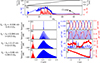Figure 3 Optical frequency comb generation dynamics. In (a) we report the laser cavity detuning, while in (b) the intra-cavity energy of the FF (blue) and SH (red) fields. In the bottom part of the figure, we report the snapshots for different spectral (c,e,g,i) and temporal (d, f, h, j) OFC regimes: (c, d) OPO, (e, f) modulation instability, (g, h) chaos and (i, j) a FF CS coupled to a SH dispersive wave.

Figure 3b shows the energy stored in the cavity versus the total number of round trips, in the different energy scales associated with waves A (E _A ) and B (E _B ). These are computed as the fast-time integral of the intra-cavity intensities |A|² and |B|²:$$E_A={\int }_{-t_{\mathrm{R}}/2}^{t_{\mathrm{R}}/2}\mathrm{}|A{|}^2\mathrm{d}\tau .$$(8)

These two quantities differ by about three orders of magnitude, being most of the power carried in the spectral domain around the driving wavelength λ₀. Nonetheless, we can notice an important energy build-up of the FF wave while δ increases and we approach the resonance condition. Above a certain power threshold, a chaotic transition clearly arises and, accordingly, we observe a chaotic nonlinear coupling to the SH domain. Finally, the emergence of a step indicates the likely excitation of a CS regime.

To sustain these statements and fully describe the comb generation, Figure 3 shows four different snapshots of the intra-cavity field (Figs. 3d, 3f, 3h, 3j) and their corresponding spectra (Figs. 3c, 3e, 3g, 3i). In Figures 3c and 3d, the system is in a blue-detuned regime but close to a resonance condition (λ_P − λ₀ = −34 pm). We observe a parametric oscillation which couples efficiently the two spectral domain ω₀ ⇆ 2ω₀. In Figure 3d, we can observe how the two waves have opposite phases. As the detuning increases and bandwidth broadens, the phase drift between the periodic patterns at ω₀ and 2ω₀ can be read as a signature of the non-zero walk-off which is detrimental to synchronize the dynamical evolution in the two separate spectral domains. Notably, typical SH powers are at a mW level, while the FF wave is three orders of magnitude more powerful (∼1 W), and the same conclusion can be drawn for the other reported OFC regimes. Increasing the detuning (λ_P − λ₀ = 86 pm), we can observe, in Figures 3e and 3f, a MI regime and the associated primary comb. The FF wave dominates the resulting dynamics, as the envelope A forms a periodic pattern while B is slaved to it. In the chaotic regime (λ_P − λ₀ = 170 pm, Figs. 3g and 3h), similarly, most of the power is carried by the FF wave and is chaotically coupled to the SH domain. Finally, Figures 3i and 3j show the final excited comb state (for a detuning λ_P − λ₀ = 860 pm). This consists of a single FF cavity soliton which, due to efficient SHG, couples part of the intracavity power around the SH. Thus the resulting dynamics consists of a single CS confined around the FF and coupled to a dispersive wave at SH. The anomalous dispersion around ω₀ (β_2,FF < 0) sustains the soliton propagation. On the other hand, normal dispersion at 2ω₀ (β_2,SH > 0) does not allow for temporal confinement of the spectral components in the SH domain. As a consequence, all the power converted at 2ω₀ by the FF CS is rapidly dispersed by the system.

Therefore, the generation of bicolor CSs [12] in the AlGaAs-on-insulator (AlGaAs-OI) platform at telecom wavelengths is intrinsically limited by the normal dispersion profile at shorter wavelengths (i.e. around 2ω₀). This is a direct consequence of the absorption peak close to the SH wavelength λ_SH = 0.775 μm. Notably, a pumping scheme λ_P ∼ 1.95 μm for a SHG assisted supercontinuum generation has been recently proposed [57]. In this specific case, supposing that a phase matching condition for the process ω₀ ⇆ 2ω₀ is satisfied, the dispersion profile is optimal at both ω₀ and 2ω₀, see Figure 2f. As a consequence, the generation of bicolor CSs is not just possible, but it also represents a strong dynamical attractor.

In a telecom pumping scheme, a suitable solution consists in engineering the chromatic dispersion, for instance by a proper longitudinal modification of the waveguide profile [40, 41], which introduces local mirroring effects and frequency splittings that are exploitable for dispersion management. Recently, some prototypes of rings [42, 58] or Fabry-Perot [59, 60] resonators of this sort have been reported.

An alternative approach could involve decoupling the nonlinear problem χ⁽²⁾ + χ⁽²⁾, by designing two separate photonic devices, which should be eventually integrated in a single circuit. An example can be a pure Kerr microring with a SHG optical feedback. With this solution in mind, let us proceed to describe an optimal AlGaAs waveguide design for efficient frequency doubling.

4 U-shaped AlGaAs waveguide design for efficient frequency doubling

If we aim at narrow-band SHG without caring about dispersive effects, we can target the PM condition between the TE₀₀ and TM₀₀ modes [22] with no further constraints on the waveguide cross-section. This approach enhances the nonlinear process thanks to the larger overlap integral between fundamental modes. This process can be generalized by letting the waveguide turn and be wrapped in a snaky fashion [47]. The scheme of the problem is depicted in Figure 4a, where we show a U-shaped waveguide with a TE₀₀ mode excited at λ₀ = 1.55 μm and phase-matched to the TM₀₀ mode at its SH. The design must optimize SHG all along the waveguide. For this reason, the waveguide width w₀ in the straight section differs from the the width w₁ of the curved section, so as to preserve the modal-PM and $\overline{4}$-QPM conditions, respectively. Specifically, type-I modal PM arises whenever the difference of the effective indices Δn_eff corresponding to the interacting modes is null, i.e. Δn_eff = 0. In a curved section, the condition for PM takes into account the difference between the azimuthal orders, i.e. Δm = 2m_FF − m_SH = ±2.

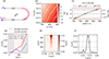Figure 4 (a) Scheme of U-shape waveguide design for frequency doubling. (b) Color map of the azimuthal number difference Δm between the TE00 mode at ω0 and the TM00 mode at 2ω0. (c) Δm vs the waveguide width for height h = 110 nm. Modal PM and $\overline{4}$-QPM conditions are reported in red and gray dashed line, respectively, while the markers correspond to PM. (d) Fraction of the power converted from FF to SH. The red line refers to the optimal situation where a change of the waveguide width enables to fulfill the $\overline{4}$-QPM condition in the curved section. The blue dashed line considers a constant width through the whole trajectory. (e) Spectral evolution of ISHG. (f) Asymmetric SHG spectrum of a U-shaped χ(2) waveguide.

From the map of Δm vs. h and w reported in Figure 4b, we can see that typical waveguide sections for phase matching between TE₀₀ (ω) and TM₀₀ (2ω) modes are much shallower than those considered above for h = 400 nm. Specifically, we note a more pronounced aspect ratio which tends to a quite-planar waveguide (h ≪ w). The resulting guided modes have typically steep dispersion profiles which are hardly manageable in a broadband domain.

Let us now set, for convenience, h = 110 nm. The resulting Δm vs. w diagram is reported in Figure 4c, which shows the $\overline{4}$-QPM and MPM conditions. The intersection with the black dashed line determines the corresponding PM widths for w₀ and w₁. Interestingly, they differ by about hundreds nm, which means that changing the waveguide width in the straight-to-curved section transition may significantly improve the SH conversion.

In order to show that, let us calculate the SHG intensity I_SHG under the undepleted-pump approximation. We suppose two straight arms of 100 μm connected by an arc of radius R = 50 μm. Figure 4d shows the two cases: I) both the modal PM and $\overline{4}$-QPM conditions are respected in the straight and the curved section, respectively (with phase matched widths w₀ ≠ w₁); II) the modal-PM condition is satisfied in the two straight sections, but the $\overline{4}$-QPM condition is not fulfilled in the arc section and the width is kept constant (w₀ = w₁). To take into account the dependence of κ on Δm, namely κ = κ(Δm), we calculate the resulting accumulated phase ϕ between the interacting modes TE₀₀ (ω) and TM₀₀ (2ω) along the propagation trajectory in equation (1), i.e. κ = κ(ϕ(Δm)). In the plot we show the fraction of converted power I_SHG/I₀, being I₀ the driving field intensity, as a function of the propagation length x. We can see that the parabolic trend of the SH intensity buildup is preserved in the straight arms for the two cases, since the modal PM condition is fulfilled. In the curved section, the typical QPM trend occurs for case I [61], while I_SHG/I₀ goes down for case II (phase mismatch).

Interestingly, in the ideal case where PM is satisfied all along a U-shaped lossless waveguide, the net power conversion is ∼16% for a total propagation length of just ∼300 μm. It is worth mentioning that, in the seek of maximizing the SHG efficiency, it is crucial to consider realistic pump depletion and optical losses, here neglected for simplicity. While this will be dealt with in future work, for the moment we may clearly state that AlGaAs may lead to an efficient ω₀ → 2ω₀ on-chip conversion in an integrated circuit with minimal propagation length.

4.1 SHG spectral symmetry breaking

Besides the monochromatic frequency conversion ω₀ → 2ω₀, if we aim to integrate the χ⁽²⁾ U-shaped waveguide in a compact χ⁽²⁾ + χ⁽³⁾ device, it is important to estimate the spectral dependence of the frequency doubling process. This can be done if we calculate the chromatic dependence of the total accumulated phase between the interacting modes TE₀₀ and TM₀₀, all along the propagation trajectory. The resulting expression for the SHG efficiency of equation (1) now takes the form κ = κ(ϕ(Δm, λ)). Notably, the dependence of the accumulated phase ϕ(Δm, λ) on Δm and λ differs between the straight and the curved sections, given that Δm has a strict waveguide width dependence (namely, Δm = Δm(w)). In what follows we compute the spectral dependence of the U-shaped design, phase-matched in both the straight and curved section.

The results of these calculations, reported in Figures 4e and 4f, are again performed under the undepleted-pump approximation. In Figure 4e, we report the 3D color map of the total intensity I_SHG converted around the SH vs the propagation length x and the wavelength λ, normalized to the driving field intensity I₀. The spectrum of I_SHG(x, λ) is clearly peaked at the SH wavelength λ₀/2, for which the constructive power build-up is guaranteed by the design, all along the U-shaped waveguide. On the contrary, we have not expressly optimized the conversion for the adjacent wavelengths, since it could possibly attenuate the conversion at λ₀/2. The resulting SH narrow-band power build-up exhibits an unclear behavior which is not necessarily constructive in the whole spectral domain and along the whole waveguide length. Moreover, a spectral asymmetry is evident with respect to the typical sinc² shape [61]. This is even more evident in the plot of the final I_SHG in Figure 4f. Here the sinc² symmetry breaking is due to the fact that, to preserve a constructive power build-up at λ₀/2, we change the waveguide width w₀ → w₁ while switching from the straight to the curved section. This responds to the quest of fulfilling both the MPM and $\overline{4}$-QPM conditions, respectively. While doing that, we span Δm over the narrow-band SHG spectrum, spanning also over different partially constructive interference conditions. As a result, the symmetry of the sinc² SH generated intensity, resulting from a straight propagation through a χ⁽²⁾ phase-matched waveguide, is broken in a U-shaped geometry where PM is granted all along the waveguide at λ₀/2.

In perspective, it is interesting to note how a wrapped snaking waveguide, composed by different U-shaped sections optimized for different SHG wavelengths, could be designed to optimize a broad-band or comb-like SHG spectrum.

5 Fabrication process

The technology we have developed to fabricate AlGaAs-OI waveguides [62] is based on adhesive bonding [17, 63] between a GaAs substrate, with the desired epitaxy of AlGaAs on top, and a thermally oxidized Si carrier wafer (see Figs. 5a–5d, for the entire process).

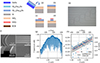Figure 5 (a–d) Fabrication process: (a) adhesive bonding of the AlGaAs epitaxy on a silicon substrate; (b) GaAs substrate removal; (c) HSQ resist spun and patterned by electron beam lithography; (d) ICP RIE etching; (e) Ring resonators and bus waveguides; (f) SEM pictures of fabricated devices: (top left) bus waveguide and ring resonator in the evanescent coupling region; (top right) fabrication test of longitudinal corrugated PhC waveguides for dispersion engineering; (bottom left) waveguide end facet; (bottom right) SW grating coupler. (g) Optical transmission of a ring resonator and (h) its associated group index n g , calculated for each resonances (blue scatters) and fitted in function of λ (red dashed line).

In Figure 5a, we schematize the bonding process. The AlGaAs epitaxy is grown by molecular beam epitaxy (MBE) on a (100) GaAs substrate and it consists of two layers: an active Al_0.18Ga_0.82As membrane (400 or 110 nm, depending on the design) and a sacrificial Al_0.8Ga_0.2As etch-stop layer. A SiO₂ layer is then deposited on the AlGaAs wafer to improve adhesion in the following bonding process. A thin benzocyclobutene (BCB) layer is spin coated on the thermal SiO₂ (2 μm) of the Si carrier, and then the AlGaAs wafer is back-flipped on it. The bonding is carried out by applying pressure and heat.

The 350 μm-thick GaAs substrate is removed in two steps using a citric acid/hydrogen peroxide solution (volume ratio 5:1): the first one at 60 °C to rapidly remove most of the substrate, the second one at 20 °C to remove the last 50 μm at a slower etch rate to minimize the tolerances due to the etching process. The sample is then rinsed in deionized water and quickly cleaned with HCl [22]. The etch-stop layer is removed using a buffered oxide solution (BOE 7:1). The result of this process is sketched on Figure 5b.

After the substrate removal, a thin SiO₂ protective layer is deposited on the Al_0.18Ga_0.18As membrane. The e-beam lithography (EBL) is carried out using hydrogen silsesquioxane (HSQ) resist (Fig. 5c). Finally, the patterns are transferred to the semiconductor membrane by ICP-RIE using a SiCl₄/Ar gas mixture (Fig. 5d).

With this process we fabricated optical waveguides and ring resonators (Figs. 5e and 5f). In Figure 5e, we show a set of micro-rings with a radius R = 50 μm with bus waveguides wrapping around to optimize the evanescent coupling. In Figure 5f, we show four scanning electron microscope (SEM) pictures: two narrow coupled waveguides (top left), PhC waveguides for dispersion management [40] (top right), a waveguide facet (bottom left) and sub-wavelength (SW) grating couplers [64] (bottom right).

5.1 Experimental characterization

The nonlinear characterization of the structures described in this paper is currently in progress and it will be the object of future work. In Figures 5g and 5h we report a preliminary linear characterization of a ring resonator. The particular bell shape of the transmission spectrum (Fig. 5g) is due to SW grating couplers used to inject and to extract light into/from the chip. We notice a good extinction ratio, which indicates the vicinity to the critical coupling condition. We estimated quality factors of around ∼10⁵. We measured a group index (Fig. 5h) consistent with the designed dispersion profile. The associated group velocity dispersion β₂ ∼ −2.5 ps²/m around the pump wavelength confirms the prescribed anomalous dispersion regime, suitable for solitons generation.

6 Conclusion and perspectives

While OFCs are deeply studied in either purely quadratic [1–3, 32] or Kerr [4, 5, 7, 17, 18, 50, 53] systems, only recently mixed χ⁽²⁾ + χ⁽³⁾ nonlinear passive resonators have been conceptualized and demonstrated [10–12, 30, 37, 38], thanks to key technological advances leading to the possibility of efficient nonlinear micro-photonics integration [55, 65]. In this work, we have proposed and discussed the perspective impact of AlGaAs for χ⁽²⁾ + χ⁽³⁾ nonlinear photonics at the telecom wavelengths. We found that Kerr-like cavity solitons can be formed and coupled to dispersive waves at SH, which tends to disperse most of the SH power. For broadband SHG applications, this represents a detrimental effect that is due to steep and hardly manageable dispersion profiles at 2ω₀. Dispersion engineering [41, 42, 44, 58, 59] and inverse design [40, 43] approaches represent a valid perspective solution and it is currently under investigation.

A possible alternative is decoupling the χ⁽²⁾ + χ⁽³⁾ nonlinear problem and to design a Kerr nonlinear resonator with a purely quadratic SHG optical feedback. We have presented a U-shaped χ⁽²⁾ design which is capable of about ∼16% ω₀ → 2ω₀ conversion with a minimal propagation length (∼300 μm).

Interestingly, we have predicted a spectral symmetry breaking due to the spanning over different phase matching conditions, in a U-shaped or snaking waveguide geometries. Notably, symmetry breaking is a key concept in physics: besides being the basic mechanism for energy-to-mass conversion in Gauge theory [66], in the field of optics it is of crucial importance for spin glasses [67] or random lasers [68]. For Kerr mediums, a symmetry-breaking transition can be responsible of periodic pattern generation [69], and in the context of nonlinear passive resonators it can generate a trapping potential for CSs [70]. Eventually, symmetry can be recovered by a chirped pulse pump [8]. As a perspective, one can investigate the possibility of designing spectral potential traps, as well as broadband SHG integrated photonics.

Acknowledgments

The authors acknowledge Hamza Dely and Victor Turpaud (C2N, CNRS) for the fruitful discussions.

Funding

ANR-22-CE92-0065, DFG-505515860 (Quadcomb); EU – NRRP, NextGenerationEU (PE00000001 – program “RESTART”). LL acknowledges the support of French Agence-innovation-defense N° DGA01D22020572. The work is partly supported by the French RENATECH network.

Conflicts of interest

The authors declare no conflicts of interest.

Data availability statement

Data underlying the results presented in this paper are not publicly available but may be obtained from the authors upon reasonable request.

Author contribution statement

FR Talenti: conceptualization, theoretical modelling and simulations, design, experiments, writing; L Lovisolo: development of the technology, fabrication, design, experiments, writing; A Gerini: design, fabrication, writing; H Peng: conceptualization; P Parra-Rivas, T Hansson, Y Sun: theory and simulations; C Alonso-Ramos: fabrication and development of the technology; M Morassi, A Lemaître: AlGaAs epitaxial growth; A Harouri: wafer bonding; C Koos: project administration, funding acquisition, supervision; S Wabnitz: theory, project administration, funding acquisition, supervision, writing; L Vivien: conceptualization, development of the technology, fabrication, supervision; G Leo: project administration, funding acquisition, supervision, writing.

References

Appendix: Numerical implementation

A.1 Normalization

In the numerical implementation of the dynamics of equations (3) and (4), it is important to adapt a proper normalization. In order to minimize the computational cost and to maximize the accuracy, good prescription is that the key parameters and variables assume values close to the unity. In our simulations, we normalized the system according to the following substitutions:$$\begin{array}{c}\begin{array}{ccc}{\alpha }_1^{\mathrm{\prime }}={\alpha }_1/{\alpha }_1=1,& {\alpha }_2^{\mathrm{\prime }}={\alpha }_2/{\alpha }_1,& \Delta \equiv \delta /{\alpha }_1,\end{array}\\ \begin{array}{ccc}{t}^{\text{'}}={\alpha }_1\mathrm{Lt}/t_r,& {\tau }^{\text{'}}=\sqrt{\frac{2{\alpha }_1}{\left|{\beta }_2\right|}}\tau ,& A^{\mathrm{\prime }},B^{\mathrm{\prime }}=\sqrt{\frac{{\gamma }_1}{{\alpha }_1}}A,B,\end{array}\\ \begin{array}{cc}{\beta }_{\mathrm{FF}\left(\mathrm{SH}\right)}^{\mathrm{\prime }}=\frac{{\beta }_{\mathrm{FF}\left(\mathrm{SH}\right)}}{{\alpha }_1}, & {\beta }_{1,\mathrm{FF}\left(\mathrm{SH}\right)}^{\mathrm{\prime }}=\sqrt{\frac{2}{{\alpha }_1|{\beta }_{2,\mathrm{FF}|}}}{\beta }_{1,\mathrm{FF}\left(\mathrm{SH}\right)},\end{array}\\ \begin{array}{cc}{\beta }_{2,\mathrm{FF}\left(\mathrm{SH}\right)}^{\mathrm{\prime }}={\beta }_{2,\mathrm{FF}\left(\mathrm{SH}\right)}/\left|{\beta }_{2,\mathrm{FF}}\right|& {\gamma }_1^{\mathrm{\prime }}={\gamma }_1/{\gamma }_1=1\end{array}\\ \begin{array}{cc}{\gamma }_{\mathrm{2,12,21}}^{\mathrm{\prime }}={\gamma }_{\mathrm{2,12,21}}/{\gamma }_1,& {\kappa }^{\text{'}}=\sqrt{\frac{1}{{\gamma }_1{\alpha }_1}}\kappa ,\end{array}\\ S^{\mathrm{\prime }}=\sqrt{\frac{{\gamma }_1}{{\alpha }_1^3{L}^2}}S,\end{array}$$(A1)where we have defined the normalized detuning Δ. The resulting coupled equations are formally identically to the system of equations (3) and (4), except for the prefactor t_R/L on the LHS, which vanishes. However, subject to this substitution, the system is dimensionless and typical solutions are of the order ∼1. It follows that the machine virtual memory used is minimized, and both the CPU efficiency and accuracy are optimized.

A.2 Numerical algorithm

In our simulations we make used of a standard split-step Fourier algorithm [49, 54]. In order to illustrate the procedure, we rewrite the system according to:$$\frac{\partial \mathcal{U}}{\partial t}=\mathcal{L}\mathcal{U}+\mathcal{NU}+\mathcal{S},$$(A2)where the linear $\mathcal{L}$, nonlinear $\mathcal{N}$ and pump $\mathcal{S}$ operators are defined, in normalized units, by comparison with equations (3) and (4):$$\mathcal{U}=\left(\begin{array}{l}{A}^{\mathrm{\prime }}\\ {\mathrm{B}}^{\mathrm{\prime }}\end{array}\right),$$(A3) $$\mathcal{LU}=\left(\begin{array}{l}-{\alpha }_1^{\text{'}}-i\Delta -i\frac{{\beta }_{2,\mathrm{FF}}^{\mathrm{\prime }}}{2}\frac{{\partial }^2}{\partial {\tau \text{'}}^2},\\ -{\alpha }_2^{\text{'}}-i2\Delta -\Delta {\beta }_1^{\mathrm{\prime }}\frac{\partial }{\partial \tau \text{'}}-i\frac{{\beta }_{2,\mathrm{SH}}^{\mathrm{\prime }}}{2}\frac{{\partial }^2}{\partial {\tau \text{'}}^2}\end{array}\right)\mathcal{U},$$(A4) $$\mathcal{NU}=\left(\begin{array}{l}\left[i{\gamma }_1^{\mathrm{\prime }}\left|A^{\text{'}}{|}^2+2i{\gamma }_{12}^{\mathrm{\prime }}\right|B^{\text{'}}{|}^2\right]\mathrm{A^\text{'}}+i{\kappa }^{\text{'}}{B}^{\text{'}}{A}^{\mathrm{\text{'}*}}\\ \left[i{\gamma }_2^{\mathrm{\prime }}|B^{\text{'}}{|}^2+2i{\gamma }_{21}^{\mathrm{\prime }}|A^{\text{'}}{|}^2\right]B\text{'}+i{\kappa }^{\text{'}\mathrm{*}}{A}^{\mathrm{\prime }2}\end{array}\right),$$(A5) $$\mathcal{S}=\left(\begin{array}{l}S\text{'}\\ 0\end{array}\right).$$(A6)

The two-steps algorithm works in both the time and Fourier domain in a single discretization step Δt, which connects two consecutive instants t _k and t _k+1 = t _k  + Δt. The linear block $\partial {\mathcal{U}}_{\mathrm{L}}/\partial t=\mathcal{L}\mathcal{U}+\mathcal{S}$ is solved analytically in the Fourier domain. The field $\mathcal{U}$ is first transformed to $\tilde{\mathcal{U}}$ by a standard fast Fourier transform (FFT) numerical operator, i.e. $\tilde{\mathcal{U}}(t_k,\omega )\equiv \mathrm{FFT}\left\{\mathcal{U}\right(t_k,\tau \left)\right\}$. Then, the linear contribution to the evolution of the jth component of the field at the kth step is computed by:$${\tilde{\mathcal{U}}}_{\mathrm{L},j}(t_{k+1},\omega )={\tilde{\mathcal{U}}}_j(t_k,\omega )e^{{\tilde{\mathcal{L}}}_j\Delta t}+\frac{{\tilde{\mathcal{S}}}_j}{{\tilde{\mathcal{L}}}_j}\left(e^{{\tilde{\mathcal{L}}}_j\Delta t}-1\right).$$(A7)

This expression is valid for the two-field components j = 1, 2, and we can note that the second term on the RHS is null for j = 2. Next, we transform back ${\tilde{\mathcal{U}}}_{\mathrm{L},j}(t_{k+1},\omega )$ to the time domain by means of an inverse fast Fourier transform operation (IFFT), i.e. ${\mathcal{U}}_{\mathrm{L},j}(t_{k+1},\tau )=\mathrm{IFFT}\left({\tilde{\mathcal{U}}}_{\mathrm{L},j}\right(t_{k+1},\omega \left)\right)$. At this point, we calculate numerically the nonlinear contribution by means of a 4th order Runge-Kutta solver (RGK4) [71]:$${\mathcal{U}}_{\mathrm{N},j}(t_{k+1},\tau )=\mathrm{RGK}4\left(\mathcal{N}{\mathcal{U}}_{\mathrm{L},j}\right(t_{k+1},\tau \left)\right).$$(A8)

The two-steps (A7) and (A8) are subject to the condition that the linear $\mathcal{L}$ and nonlinear $\mathcal{N}$ operators act separately and independently on the two waves field $\mathcal{U}$. This condition is mathematically fulfilled if and only if their commutator vanishes, i.e. $\left[\mathcal{L},\mathcal{N}\right]\mathcal{U}=0$ [49]. This is true in the limit Δt → 0, and thus the accuracy of procedure crucially relies on the choice of small enough discretization steps Δt.

A.3 Dispersion effects

The contribution of chromatic dispersion effects is evaluated in the Fourier domain and embedded in the linear operator $\tilde{\mathcal{L}}\left(\omega \right)$. The system of equations (3) and (4) neglects leading order terms with respect to the GVD. Within this approximation, the operator $\tilde{\mathcal{L}}\left(\omega \right)$ reads as:$$\tilde{\mathcal{L}}\left(\omega \right)\approx \left(\begin{array}{l}-{\alpha }_1^{\text{'}}-i\Delta +i{\beta }_{2,\mathrm{FF}}^{\mathrm{\prime }}{\omega }^2\\ -{\alpha }_2^{\mathrm{\prime }}-2i\Delta -\Delta {\beta }_1^{\text{'}}\omega +i{\beta }_{2,\mathrm{SH}}^{\mathrm{\prime }}{\omega }^2\end{array}\right).$$(A9)

This approximation is optimal in a narrow band spectral domain, while for broadband dynamics can be detrimental. In our case, we have a doubly resonant system which owns spectral components covering the whole octave spanning FF → SH domain, with important dispersive effects. For this reason, the use of a full dispersion profile is of crucial importance for the implementation of reliable and realistic models. In multi-envelope systems [39], we can expand in Taylor series the propagation constant β(ω) (Eq. (2)). The standard substitution reads as [54]:$$\sum _{k\ge 2}^{\infty }\mathrm{}\frac{{\beta }_k}{k!}{\omega }^k=\beta \left(\omega \right)-{\beta }_1\omega -{\beta }_0.$$(A10)

With this procedure we can take into account leading order dispersive terms in equations (3) and (4). The full dispersion profile is thus embedded rewriting the linear operator $\tilde{\mathcal{L}}$ as:$$\tilde{\mathcal{L}}\left(\omega \right)=\left(\begin{array}{l}-{\alpha }_1^{\text{'}}-i\Delta +i\left({\beta }_{\mathrm{FF}}^{\mathrm{\prime }}\left(\omega \right)-{\beta }_{1,\mathrm{FF}}^{\text{'}}\omega -{\beta \text{'}}_{0,\mathrm{FF}}\right)\\ -{\alpha \text{'}}_2-2i\Delta +i\left({\beta }_{\mathrm{SH}}^{\mathrm{\prime }}\left(\omega \right)+({\beta }_{1,\mathrm{FF}}^{\mathrm{\prime }}-2{\beta }_{1,\mathrm{SH}}^{\mathrm{\prime }})\omega -{\beta }_{0,\mathrm{SH}}^{\mathrm{\prime }}\right)\end{array}\right).$$(A11)

A.4 Codes implementation

The numerical implementation of the dynamical models presented in this work, has been fully developed by home-built codes using Julia language [72].

All Figures

	Figure 1 (a) Scheme of a passively driven doubly resonant SHG-Kerr ring resonator. (b) Transverse cross-section with height h and width w.
In the text

Figure 2 (a) Energy density of the phase-matched guided modes at ω0 (TE00 and TM00) and 2ω0 (TE02,SH). (b) neff vs. w diagram of type-I (red marker) and type-II (blue marker) modal PM. (c) SHG efficiency as a function of the angle θ between the propagation direction and the [100] axis. (d) Effective index neff, (e) group velocity β1, and (f) GVD β2 for the TE00,FF (blue dashed line), TM00,FF (blue pointed line) and TE02,SH modes (red dashed line). In (d, e, f) the colored arrows indicate the corresponding x-axis.

In the text

Figure 3 Optical frequency comb generation dynamics. In (a) we report the laser cavity detuning, while in (b) the intra-cavity energy of the FF (blue) and SH (red) fields. In the bottom part of the figure, we report the snapshots for different spectral (c,e,g,i) and temporal (d, f, h, j) OFC regimes: (c, d) OPO, (e, f) modulation instability, (g, h) chaos and (i, j) a FF CS coupled to a SH dispersive wave.

In the text

Figure 4 (a) Scheme of U-shape waveguide design for frequency doubling. (b) Color map of the azimuthal number difference Δm between the TE00 mode at ω0 and the TM00 mode at 2ω0. (c) Δm vs the waveguide width for height h = 110 nm. Modal PM and $\overline{4}$-QPM conditions are reported in red and gray dashed line, respectively, while the markers correspond to PM. (d) Fraction of the power converted from FF to SH. The red line refers to the optimal situation where a change of the waveguide width enables to fulfill the $\overline{4}$-QPM condition in the curved section. The blue dashed line considers a constant width through the whole trajectory. (e) Spectral evolution of ISHG. (f) Asymmetric SHG spectrum of a U-shaped χ(2) waveguide.

In the text

Figure 5 (a–d) Fabrication process: (a) adhesive bonding of the AlGaAs epitaxy on a silicon substrate; (b) GaAs substrate removal; (c) HSQ resist spun and patterned by electron beam lithography; (d) ICP RIE etching; (e) Ring resonators and bus waveguides; (f) SEM pictures of fabricated devices: (top left) bus waveguide and ring resonator in the evanescent coupling region; (top right) fabrication test of longitudinal corrugated PhC waveguides for dispersion engineering; (bottom left) waveguide end facet; (bottom right) SW grating coupler. (g) Optical transmission of a ring resonator and (h) its associated group index n g , calculated for each resonances (blue scatters) and fitted in function of λ (red dashed line).

In the text

References

- Ulvila V, Phillips CR, Halonen L, Vainio M, Frequency comb generation by a continuous-wave-pumped optical parametric oscillator based on cascading quadratic nonlinearities, Opt. Lett. 38, 4281 (2013). https://doi.org/10.1364/ol.38.004281. [Google Scholar]
- Ricciardi I, et al. Frequency comb generation in quadratic nonlinear media, Phys. Rev. A. 91, 063839 (2015). https://doi.org/10.1103/physreva.91.063839. [Google Scholar]
- Leo F, et al., Walk-off-induced modulation instability, temporal pattern formation, and frequency comb generation in cavity-enhanced second-harmonic generation, Phys. Rev. Lett. 116, 033901 (2016). https://doi.org/10.1103/physrevlett.116.033901. [Google Scholar]
- Del’Haye P, Herr T, Gavartin E, Gorodetsky ML, Holzwarth R, Kippenberg TJ, Octave spanning tunable frequency comb from a microresonator, Phys. Rev. Lett. 107, 063901 (2011). https://doi.org/10.1103/physrevlett.107.063901. [Google Scholar]
- Herr T, et al., Temporal solitons in optical microresonators, Nat. Photonics. 8, 145 (2013). https://doi.org/10.1038/nphoton.2013.343. [Google Scholar]
- Wabnitz S, Suppression of interactions in a phase-locked soliton optical memory, Opt. Lett. 18, 601 (1993). https://doi.org/10.1364/ol.18.000601. [Google Scholar]
- Rowley M, et al., Self-emergence of robust solitons in a microcavity, Nature 608, 303 (2022). https://doi.org/10.1038/s41586-022-04957-x. [Google Scholar]
- Talenti FR, Sun Y, Parra-Rivas P, Hansson T, Wabnitz S, Control and stabilization of Kerr cavity solitons and breathers driven by chirped optical pulses, Opt. Commun. 546, 129773 (2023). https://doi.org/10.1016/j.optcom.2023.129773. [Google Scholar]
- Szabados J, Sturman B, Breunig I, Frequency comb generation threshold via second-harmonic excitation in χ(2) optical microresonators, APL Photonics 5, 116102 (2020). https://doi.org/10.1063/5.0021424. [CrossRef] [Google Scholar]
- Bruch AW, Liu X, Surya JB, Zou CL, Tang HX, On-chip χ(2) microring optical parametric oscillator, Optica 6, 1361 (2019). https://doi.org/10.1364/optica.6.001361. [Google Scholar]
- Bruch AW, et al., Pockels soliton microcomb, Nat. Photonics 15, 21 (2020). https://doi.org/10.1038/s41566-020-00704-8. [Google Scholar]
- Lu J, et al., Two-colour dissipative solitons and breathers in microresonator second-harmonic generation, Nat. Commun. 14, 2798 (2023). https://doi.org/10.1038/s41467-023-38412-w. [Google Scholar]
- Coudrat L, Boulliard G, Gérard JM, Lemaître A, Degiron A, Leo G, Unravelling the nonlinear generation of designer vortices with dielectric metasurfaces, Light Sci. Appl. 14, 51 (2025). https://doi.org/10.1038/s41377-025-01741-0. [Google Scholar]
- de Ceglia D, et al., Nonlinear spin-orbit coupling in optical thin films, Nat. Commun. 15, 1625 (2024). https://doi.org/10.1038/s41467-024-45607-2. [Google Scholar]
- Chopin A, et al., Ultra-efficient generation of time-energy entangled photon pairs in an InGaP photonic crystal cavity, Commun. Phys. 6, 77 (2023). https://doi.org/10.1038/s42005-023-01189-x. [Google Scholar]
- Schuhmann J, et al., Hybrid III-V/silicon quantum photonic device generating broadband entangled photon pairs, PRX Quantum. 5, 040321 (2024). https://doi.org/10.1103/prxquantum.5.040321. [Google Scholar]
- Pu M, Ottaviano L, Semenova E, Yvind K, Efficient frequency comb generation in AlGaAs-on-insulator, Optica. 3, 823 (2016). https://doi.org/10.1364/optica.3.000823. [Google Scholar]
- Chang L, et al., Ultra-efficient frequency comb generation in AlGaAs-on-insulator microresonators, Nat. Commun. 11, 1331 (2020). https://doi.org/10.1038/s41467-020-15005-5. [Google Scholar]
- Marty G, Combrié S, Raineri F, De Rossi A, Photonic crystal optical parametric oscillator, Nat. Photonics. 15, 53 (2020). https://doi.org/10.1038/s41566-020-00737-z. [Google Scholar]
- Chopin A, et al., Canonical resonant four-wave-mixing in photonic crystal cavities: tuning, tolerances and scaling, IEEE J. Sel. Top. Quantum Electron. 29, 5100913 (2022). https://doi.org/10.1109/jstqe.2022.3229164. [Google Scholar]
- Chang L, et al., Strong frequency conversion in heterogeneously integrated GaAs resonators, APL Photonics 4, 036103 (2019). https://doi.org/10.1063/1.5065533. [CrossRef] [Google Scholar]
- Stanton EJ, et al., Efficient second harmonic generation in nanopho tonic GaAs-on-insulator waveguides, Opt. Express. 28, 9521 (2020). https://doi.org/10.1364/oe.389423. [Google Scholar]
- Gerini A, et al., Second harmonic generation in monolithic GaAs shallow waveguides, Opt. Express 33, 17560 (2025). https://doi.org/10.1364/OE.540737. [Google Scholar]
- Poulvellarie N, et al., Second-harmonic generation enabled by longitudinal electric-field components in photonic wire waveguides, Phys. Rev. A. 102, 023521 (2020). https://doi.org/10.1103/physreva.102.023521. [Google Scholar]
- Ciret C, et al., Influence of longitudinal mode components on second harmonic generation in III-V-on-insulator nanowires, Opt. Express 28, 31584 (2020). https://doi.org/10.1364/oe.402150. [Google Scholar]
- Poulvellarie N, et al., Efficient type II second harmonic generation in an indium gallium phosphide on insulator wire waveguide aligned with a crystallographic axis, Opt. Lett. 46, 1490 (2021). https://doi.org/10.1364/ol.418064. [Google Scholar]
- Pantzas K, et al., Continuous-wave second-harmonic generation in orientation-patterned gallium phosphide waveguides at telecom wavelengths, ACS Photonics 9, 2032 (2022). https://doi.org/10.1021/acsphotonics.2c00156. [Google Scholar]
- Akin J, Zhao Y, Misra Y, Haque AKMN, Fang K, InGaP χ(2) integrated photonics platform for broadband, ultra-efficient nonlinear conversion and entangled photon generation, Light Sci. Appl. 13, 290 (2024). https://doi.org/10.1038/s41377-024-01653-5. [Google Scholar]
- Gerini A, et al., Electrically injected InGaAsP/AlGaAs optical parametric oscillator: design and technology, J. Opt. Soc. Am. B. 38, B40 (2021). https://doi.org/10.1364/josab.425018. [Google Scholar]
- Talenti FR, et al., Frequency comb generation dynamics in χ(2) + χ(3) AlGaAs microresonators, EPJ Web Conf. 309, 08003 (2024). https://doi.org/10.1051/epjconf/202430908003. [Google Scholar]
- Talenti FR, et al., Bistable soliton optical frequency combs in a second-harmonic generation Kerr cavity, Opt. Lett. 50, 2037 (2025). https://doi.org/10.1364/OL.551383. [Google Scholar]
- Hansson T, Parra-Rivas P, Bernard M, Leo F, Gelens L, Wabnitz S, Quadratic soliton combs in doubly resonant second-harmonic generation, Opt. Lett. 43, 6033 (2018). https://doi.org/10.1364/ol.43.006033. [Google Scholar]
- Leo F, et al., Frequency-comb formation in doubly resonant second-harmonic generation, Phys. Rev. A. 93, 043831 (2016). https://doi.org/10.1103/physreva.93.043831. [Google Scholar]
- Hansson T, Parra-Rivas P, Wabnitz S, Modeling of dual frequency combs and bistable solitons in third-harmonic generation, Commun. Phys. 6, 59 (2023). https://doi.org/10.1038/s42005-023-01176-2. [Google Scholar]
- Trillo S, Wabnitz S, Nonlinear parametric mixing instabilities induced by self-phase and cross-phase modulation, Opt. Lett. 17, 1572 (1992). https://doi.org/10.1364/ol.17.001572. [Google Scholar]
- Buryak AV, Trillo S, Kivshar YS, Optical solitons supported by competing nonlinearities, Opt. Lett. 20, 1961 (1995). https://doi.org/10.1364/ol.20.001961. [Google Scholar]
- Villois A, Kondratiev N, Breunig I, Puzyrev DN, Skryabin DV, Frequency combs in a microring optical parametric oscillator, Opt. Lett. 44, 4443 (2019). https://doi.org/10.1364/ol.44.004443. [Google Scholar]
- Xue X, et al., Second-harmonic-assisted four-wave mixing in chip-based microresonator frequency comb generation, Light Sci. Appl. 6, e16253 (2016). https://doi.org/10.1038/lsa.2016.253. [Google Scholar]
- Phillips CR, Jankowski M, Flemens N, Fejer MM, General framework for ultrafast nonlinear photonics: unifying single and multi-envelope treatments, Opt. Express. 32, 8284 (2024). https://doi.org/10.1364/oe.513856. [Google Scholar]
- Talenti FR, Wabnitz S, Ghorbel I, Combrié S, Aimone-Giggio L, De Rossi A, Fast dispersion tailoring of multimode photonic crystal resonators, Phys. Rev. A. 106, 023505 (2022). https://doi.org/10.1103/physreva.106.023505. [Google Scholar]
- De Rossi A, Combrié S, The dawn of chimera optical resonators, Nat. Photonics 18, 112 (2024). https://doi.org/10.1038/s41566-023-01376-w. [Google Scholar]
- Moille G, Lu X, Stone J, Westly D, Srinivasan K, Fourier synthesis dispersion engineering of photonic crystal microrings for broadband frequency combs, Commun. Phys. 6, 144 (2023). https://doi.org/10.1038/s42005-023-01253-6. [Google Scholar]
- Gray D, West GN, Ram RJ, Inverse design for waveguide dispersion with a differentiable mode solver, Optics Express. 32, 30541 (2024). https://doi.org/10.1364/oe.530479. [Google Scholar]
- Lucas E, Yu SP, Briles TC, Carlson DR, Papp SB, Tailoring microcombs with inverse-designed, metadispersion microresonators, Nat. Photonics 17, 943 (2023). https://doi.org/10.1038/s41566-023-01252-7. [Google Scholar]
- Abolghasem P, Han JB, Kang D, Bijlani BJ, Helmy AS, Monolithic photonics using second-order optical nonlinearities in multilayer-core Bragg reflection waveguides, IEEE J. Sel. Top. Quantum Electron. 18, 812 (2011). https://doi.org/10.1109/JSTQE.2011.2135841. [Google Scholar]
-
Kuo PS, Fang W, Solomon GS,
-quasi-phase-matched interactions in GaAs microdisk cavities, Opt. Lett. 34, 3580 (2009). https://doi.org/10.1364/ol.34.003580.
[Google Scholar]
- Morais N, et al., Directionally induced quasi-phase matching in homogeneous AlGaAs waveguides, Opt. Lett. 42, 4287 (2017). https://doi.org/10.1364/ol.42.004287. [Google Scholar]
- Ansys (Lumerical Inc, 2000). Available at https://www.lumerical.com/. [Google Scholar]
- Agrawal GP, Nonlinear fiber optics (Springer, Berlin, Heidelberg, 2000). [Google Scholar]
- Pasquazi A, et al., Micro-combs: A novel generation of optical sources, Phys. Rep. 729, 1 (2018). https://doi.org/10.1016/j.physrep.2017.08.004. [Google Scholar]
- Laegsgaard J, Mode profile dispersion in the generalised nonlinear Schrödinger equation, Opt. Express. 15, 16110 (2007). https://doi.org/10.1364/oe.15.016110. [Google Scholar]
- Buryak AV, Trapani PD, Skryabin DV, Trillo S, Optical solitons due to quadratic nonlinearities: from basic physics to futuristic applications, Phys. Rep. 370, 63 (2002). https://doi.org/10.1016/s0370-1573(02)00196-5. [CrossRef] [MathSciNet] [Google Scholar]
- Hansson T, Wabnitz S, Dynamics of microresonator frequency comb generation: models and stability, Nanophotonics. 5, 231 (2016). https://doi.org/10.1515/nanoph-2016-0012. [Google Scholar]
- Dudley JM, Taylor JR, Supercontinuum generation in optical fibers (Cambridge University Press, Cambridge, 2010). [CrossRef] [Google Scholar]
- Leuthold J, Koos C, Freude W, Nonlinear silicon photonics, Nat. Photonics. 4, 535 (2010). https://doi.org/10.1038/nphoton.2010.185. [Google Scholar]
- Lin Q, Painter OJ, Agrawal GP, Nonlinear optical phenomena in silicon waveguides: modeling and applications, Opt. Express. 15, 16604 (2007). https://doi.org/10.1364/oe.15.016604. [Google Scholar]
- Nishi H, Sugiyama H, Kanno E, Segawa T, Wada K, Matsuo S, Second-harmonic-wave assisted octave-spanning supercontinuum generation in an AlGaAs-on-insulator waveguide, in: 2024 IEEE Silicon Photonics Conference (SiPhotonics), 15–18 April, Tokyo Bay, Japan (IEEE, 2024), p. 1. https://doi.org/10.1109/siphotonics60897.2024.10543509. [Google Scholar]
- Yu SP, Lucas E, Zang J, Papp SB, A continuum of bright and dark-pulse states in a photonic-crystal resonator, Nat. Commun. 13, 3134 (2022). https://doi.org/10.1038/s41467-022-30774-x. [Google Scholar]
- Yu SP, Jung H, Briles TC, Srinivasan K, Papp SB, Photonic-crystal-reflector nanoresonators for kerr-frequency combs, ACS Photonics 6, 2083 (2019). https://doi.org/10.1021/acsphotonics.9b00578. [Google Scholar]
- Wildi T, Gaafar MA, Voumard T, Ludwig M, Herr T, Dissipative Kerr solitons in integrated Fabry–Perot microresonators, Optica 10, 650 (2023). https://doi.org/10.1364/optica.480789. [Google Scholar]
- Boyd RW, Gaeta AL, Giese E, Nonlinear optics (Springer, New York, 2008). [Google Scholar]
- Mobini E, Espinosa DHG, Vyas K, Dolgaleva K, AlGaAs nonlinear integrated photonics, Micromachines 13, 991 (2022). https://doi.org/10.3390/mi13070991. [Google Scholar]
- May S, Clerici M, Sorel M, Supercontinuum generation in dispersion engineered AlGaAs-on-insulator waveguides, Sci. Rep. 11, 2052 (2021). https://doi.org/10.1038/s41598-021-81555-3. [Google Scholar]
- Halir R, et al., Waveguide sub-wavelength structures: a review of principles and applications, Laser Photonics Rev. 9, 25 (2014). https://doi.org/10.1002/lpor.201400083. [Google Scholar]
- Vermeulen N, et al., Post-2000 nonlinear optical materials and measurements: data tables and best practices, J. Phys. Photonics 5, 035001 (2023). https://doi.org/10.1088/2515-7647/ac9e2f. [Google Scholar]
- Higgs PW, Broken symmetries and the masses of gauge bosons, Phys. Rev. Lett. 13, 508 (1964). https://doi.org/10.1103/physrevlett.13.508. [Google Scholar]
- Parisi G, The order parameter for spin glasses: a function on the interval 0–1, J. Phys A: Math. General. 13, 1101 (1980). https://doi.org/10.1088/0305-4470/13/3/042. [Google Scholar]
- Massaro LM, et al., Heterogeneous random laser with switching activity visualized by replica symmetry breaking maps, ACS Photonics 8, 376 (2021). https://doi.org/10.1021/acsphotonics.0c01803. [Google Scholar]
- Ducci S, Ramazza PL, González-Viñas W, Arecchi FT, Order parameter fragmentation after a symmetry-breaking transition, Phys Rev Lett. 83, 5210 (1999). https://doi.org/10.1103/PhysRevLett.83.5210. [Google Scholar]
- Hendry I, et al., Spontaneous symmetry breaking and trapping of temporal Kerr cavity solitons by pulsed or amplitude-modulated driving fields, Phys. Rev. A. 97, 053834 (2018). https://doi.org/10.1103/physreva.97.053834. [Google Scholar]
- Butcher JC, A history of Runge-Kutta methods, Appl. Numer. Math. 20, 247 (1996). https://doi.org/10.1016/0168-9274(95)00108-5. [Google Scholar]
- Bezanson J, Edelman A, Karpinski S, Shah VB, Julia: A fresh approach to numerical computing, SIAM Rev. 59, 65 (2017). https://doi.org/10.1137/141000671. [CrossRef] [Google Scholar]