| Issue |
J. Eur. Opt. Society-Rapid Publ.
Volume 22, Number 1, 2026
|
|
|---|---|---|
| Article Number | 32 | |
| Number of page(s) | 15 | |
| DOI | https://doi.org/10.1051/jeos/2026027 | |
| Published online | 07 May 2026 | |
Research Article
Research on the evolution law of ship targets infrared characteristics in port environment
1
Shaanxi University of Science & Technology, Xi’an 710021, PR China
2
School of Physics, Xidian University, Xi’an 710071, PR China
* Corresponding author: This email address is being protected from spambots. You need JavaScript enabled to view it.
Received:
20
January
2025
Accepted:
7
March
2026
Abstract
Based on the differences in material properties between the target and the background, and combined with changes in environmental, lighting, and temporal conditions, an optical imaging feature prediction model for ship targets in a port background is constructed to explore the impact of the “thermal crossover” phenomenon on the infrared detection performance of ship targets. Firstly, Fluent software is used to calculate the surface temperature distribution of the target under different environmental conditions. Combined with the material and radiation scattering characteristics of different parts of the target, a radiation transmission model of the ship target is constructed. Secondly, Landsat 8 remote sensing data is used to invert the port temperature distribution under specific seasonal and temporal conditions, and land cover classification is performed based on a supervised classification algorithm. Based on meteorological data, the Kriging algorithm is used to achieve temperature expansion of the port background under different temporal conditions. Meanwhile, topographic factors such as elevation, slope, and aspect of land features are taken into account to establish a high-precision temporal temperature reconstruction model with topographic modulation. The differences in sea surface radiation characteristics and scattering effects are taken into account to establish a background radiation transfer model. Finally, combining solar, sky, and atmospheric radiative transfer models, the modulation effect of the space-based optical platform is considered, and an imaging prediction model of the “ship target-port background-ambient illumination-atmospheric transmission” is established. The results show that during non-thermal crossover periods in summer, the detectability of 3–5 μm is better than that of 8–14 μm, while the opposite is true during thermal crossover periods in winter. At the critical moment of thermal crossover in summer, the detectability of 3–5 μm is worse than that of 8–14 μm, while at the critical moment of thermal crossover in winter, the detectability of 3–5 μm and 8–14 μm are relatively close.
Key words: Thermal crossover / Infrared radiation and imaging / Modeling and simulation / Space-based detection
© The Author(s), published by EDP Sciences, 2026
 This is an Open Access article distributed under the terms of the Creative Commons Attribution License (https://creativecommons.org/licenses/by/4.0), which permits unrestricted use, distribution, and reproduction in any medium, provided the original work is properly cited.
1 Introduction
A deep understanding of the infrared characteristics of ships is not only the foundation for improving the accuracy of infrared imaging simulation, but also a key prerequisite for realizing automatic target identification and threat assessment [1]. Space-based infrared detection has important application value in maritime monitoring, early warning and target identification [2]. However, the imaging results from the space-based platforms are affected by multiple factors such as complex background, atmospheric transmission and optical system characteristics. Especially in the typical scenario of a port, the dense ship targets, complex background composition, and frequent environmental changes lead to a significant dynamic evolution of the infrared characteristics of the targets.
Accurate understanding of the space-based optical imaging characteristics of ship targets has always been an important research direction in the field of infrared detection. Many scholars have conducted fruitful research work in this area, and related theories and methods are constantly being improved. The surface temperature and the IR signals within MWIR and LWIR are calculated considering the 3D ship model, the internal heater temperature, and the atmospheric conditions [3]. Bin C [4] studied the infrared simulation of warships under different statuses and simulated the ship wake, and proposed a wake modeling method, which improved the fidelity of the whole scene. A ship infrared radiation calculation model is proposed by LIN Juan [5] based on the infrared radiation rendering of solid targets, which considers the spontaneous radiation and environmental radiation of ships. The infrared simulation results are compared and verified based on experimental data. The simulation calculation of focal plane radiation characteristics for ship target is realized based on the full chain of optical remote sensing detection. The ship target radiation characteristics under different sea surface conditions and different imaging time are analyzed by Z Jiang [6]. Zhang C W [7] proposed a high-frequency method by using graphics processing unit (GPU) parallel acceleration technique, simulated signals of ships at different seas. Wang M [8] proposed a data-driven infrared radiation modeling method, which optimizes the model accuracy by comparing measured data with theoretical models, and is used to simulate the infrared characteristics of marine targets under typical sea conditions. Song Bo [9] proposed a high-resolution remote sensing imaging simulation method for marine targets, focusing on the simulation method of the imaging process of the coupling effect between sea surface targets and seawater under high resolution. Jiang Le et al. [10, 11] comprehensively considered the influence of environmental factors on the infrared radiation characteristics of the target and explored the radiation modeling and simulation method of infrared scene. Meanwhile, some scholars have also explored methods for calculating the radiation characteristics of ship targets [12, 13] and simulation methods for high-confidence infrared background imaging characteristics [14, 15], providing a theoretical basis for the simulation of infrared characteristics and exploration of characteristic laws of typical targets.
The above research has made significant progress in understanding the infrared characteristics of ships, but the following shortcomings still exist. The complex port environment is affected by the diurnal cycle, variations in solar radiation, and the difference in thermal inertia between land and sea. The infrared radiation characteristics of the target and background may tend to be consistent or even reversed at certain times. This phenomenon is called “thermal crossover.” Existing research on ship infrared imaging simulation generally ignores the “thermal crossover” phenomenon caused by the dynamic changes in heat exchange under complex port backgrounds, making it difficult to accurately depict the temporal evolution of the infrared contrast of ship targets and background under space-based conditions. The problem essentially stems from the coupling and reversal relationship between the target and background temperatures over time, and there is an urgent need to establish a physical modeling framework that can accurately describe its time-varying characteristics. Although some scholars have used remote sensing data to model the background temperature [16–18] or used deep learning methods to extrapolate the spatiotemporal characteristics of background radiation [14, 15], the applicability of their results in complex scenarios is still limited due to the temporal constraints of the data and the insufficient physical interpretability of the models [19–21]. Therefore, if research on radiation coupling modeling of targets and backgrounds under time-series conditions is carried out, it will be of great significance for revealing the evolution law of ship infrared characteristics and improving the realism of imaging simulation.
To address the shortcomings of previous research, a spatiotemporal reconstruction method for the port background temperature, which integrates meteorological data and topographic features based on Landsat 8 remote sensing data, is proposed in this paper. First, based on environmental meteorological data, the Kriging algorithm is used to achieve a preliminary expansion of surface temperature under different temporal conditions. Then, topographic factors such as elevation, slope, and aspect are taken into account to establish a modulation model for surface radiation balance and energy exchange. Last, the background temperature is finely corrected and reconstructed with high precision. This method effectively improves the spatial continuity and physical consistency of surface temperature retrieval, providing reliable support for the simulation of ground feature background and environmental change analysis in complex terrain areas.
2 Port infrared scene modeling
From a space-based platform, the background includes not only the water surface and dock facilities, but is also subject to complex influences from atmospheric conditions, weather changes, and environmental heat sources. To reflect the radiation distribution in a real environment, a method of inverting remote sensing data to obtain the port background temperature field is used, and the infrared characteristics of different surfaces such as the sea surface, cement wharf, and building facilities are modeled to achieve high-precision characterization of multi-source background radiation. Figure 1 is a schematic diagram of the space-based optoelectronic system detecting targets.
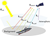 |
Figure 1 Space-based optoelectronic system detecting targets. |
The total scene radiation distribution received by the detector [22] can be expressed as:![Mathematical equation: $$ {L}_{sensor}\left(\lambda \right)={\tau}_a\left[{L}_t^{\uparrow}\left(\lambda \right)+{L}_b^{\uparrow}\left(\lambda \right)\right]+{L}_a^{\uparrow}\left(\lambda \right) $$](/articles/jeos/full_html/2026/01/jeos20260006/jeos20260006-eq1.gif) (1)
(1)
where τa is the atmospheric upward transmittance; L↑t is the target upward radiation; L↑b is the background upward radiation; and L↑a is the atmospheric path upward radiation. The total background radiation includes its own radiation and reflected radiation. It is necessary to classify the background materials and establish radiative transfer models for different materials. The port background includes ocean and land, the total background radiance [22] can be expressed as:![Mathematical equation: $$ {L}_b\left(\lambda \right)={L}_{b, self}^{\uparrow}\left(\lambda \right)+{L}_{b, ref}^{\uparrow}\left(\lambda \right)=\frac{\varepsilon_b\left(\lambda \right)}{\pi }{\int}_{\lambda_1}^{\lambda_2}\frac{c_1}{\left[\exp \left({c}_2/{\lambda T}_b\right)-1\right]} d\lambda +{\tau}_s{E}_{sun}\cos {\theta}_i{BRDF}_b\left({\theta}_i,{\varphi}_{i,}{\theta}_r,{\varphi}_r\right)+{\rho}_b\cdot {L}_{sky} $$](/articles/jeos/full_html/2026/01/jeos20260006/jeos20260006-eq2.gif) (2)
(2)
where εb is the emissivity of different background materials; c1 is 1.191×10⁸ W/μm·sr·m2; c2 is 1.4388 × 104 μm K; Tb is the background temperature distribution; τs is the atmospheric transmittance of solar radiation to the background; Esun is the solar irradiance; BRDFb is the bidirectional reflectivity of the background; θi(φi) and θr(φr) are the incident zenith angle (incident azimuth angle) and the reflected zenith angle (reflection azimuth angle), respectively; ρb is the background reflectivity; and Lsky is the incident radiance of the sky.
2.1 Port temperature distribution inversion
Measured remote sensing images over a coastal region in northern China were selected from Landsat 8 TIRS Band 10 imagery (30 m). Surface temperature was retrieved using a single-channel algorithm [18]. Figure 2 illustrates the temperature differences between the sea surface and land in different seasons. In spring and autumn, the temperature difference between the sea and land is small, and the temperature changes are stable. The land surface heats up quickly in summer and cools down quickly in winter. Seawater, due to its high specific heat capacity, experiences smaller temperature fluctuations.
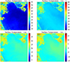 |
Figure 2 The temperature distribution of the four seasons in the port. (a) Spring. (b) Summer. (c) Autumn. (d) Winter. |
Due to the significant differences in the radiation characteristics of different land cover types and sea surfaces, it is necessary to establish corresponding radiation characteristic models for various land types to improve the physical consistency and accuracy of the inversion results. In addition, due to the limitations of the spatiotemporal resolution of satellite observations, the inversion results only reflect the temperature distribution at a specific transit time. It is difficult to directly characterize the changes in thermal radiation throughout the day or over a continuous period of time. Therefore, it is necessary to extend the temperature time series to obtain multi-temporal temperature fields.
2.2 Port background feature classification
To improve the accuracy of infrared radiation calculation for port backgrounds, a supervised classification method is used to classify the background features. First, the original image needs to undergo preprocessing such as radiometric calibration, atmospheric correction, and cropping. Then, regions of interest (ROIs) are established to select training samples for each category, and the ROIs for each type of feature are marked with different colors. Figure 3 illustrates the supervised classification process.
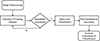 |
Figure 3 The supervised classification process. |
The separability between different sample types is determined by calculating the Jeffries-Matusita Distance (JM) and the transformation separation. A maximum likelihood-based classification is selected for sample training to generate a classification model, which is then processed. At last, the accuracy and reliability of the classification are measured by two indicators: the overall accuracy in the confusion matrix and the Kappa coefficient. The JM distance [23] can be expressed as: (3)
(3)![Mathematical equation: $$ B=\frac{1}{8}{\left({m}_1-{m}_2\right)}^2\frac{2}{\sigma_1^2+{\sigma}_2^2}+\frac{1}{2}\left[\ln \right]\left[\frac{\sigma_1^2+{\sigma}_2^2}{2{\sigma}_1{\sigma}_2}\right] $$](/articles/jeos/full_html/2026/01/jeos20260006/jeos20260006-eq4.gif) (4)
(4)
where B is the Bhattacharyya distance between the two classes based on a certain feature, m1 and m2 are the feature means of the two classes, and σ1 and σ2 are the feature standard deviations of the two classes. The calculation results are shown below:
The JM distance range from 0 to 2, where 0 indicates that the two categories are almost completely confused on a certain feature, and 2 indicates that the two categories are completely separated on a certain feature. As shown in the Table 1, the separability values are all greater than 1.9, indicating reasonable sample separation. The images are classified according to the maximum likelihood method, and the results are shown in Figure 4.
Sample separability calculation results.
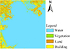 |
Figure 4 Land surface classification result. |
As shown in Figure 4, the port background features can be roughly divided into four categories, with the following percentages: water 81.54%, vegetation 2.92%, land 7.45%, and buildings 8.09%. A confusion matrix is used to evaluate the classification results, determining the accuracy and reliability of the classification. Two indicators, Overall Accuracy (OA) and Kappa Coefficient [24], are used for evaluation: (5)
(5) (6)where wi,j is the squared weighted average; Oi,j is the element in the observation matrix; Ei,j is the element in the expectation matrix; N is the total number of classifications. The classification verification results are follows, the overall accuracy is 0.9984, which is higher than 85%. Kappa Coefficient is 0.9211, which is greater than 0.8, indicating that the land cover classification is accurate.
2.3 Modeling of port background BRDF
Based on the above classification results, bidirectional reflection models can be established for land and sea surfaces respectively. Sea water surface reflection is calculated using the Cox-Munk model, taking into account the effects of wind speed, wind direction, and obstruction. The bidirectional reflection function of the sea surface [18] is expressed as: (7)where P(zu, zv) is the probability distribution of sea surface slope; ρ(ω) is the sea surface reflectivity, calculated according to Fresnel’s theorem; θr is the zenith angle of the reflection direction; β is the tilt rate of the small surface element. To accurately characterize the reflection properties of the land surface, the Rahman-Pinty-Verstraete (RPV) semi-empirical BRDF model is introduced [25], which can be expressed as:
![Mathematical equation: $$ {BRDF}_{land}\left({\theta}_i,{\theta}_v,\varphi\ \right)={r}_0\frac{\cos {\theta}_i^{k-1}-\cos {\theta}_v^{k-1}}{{\left(\cos {\theta}_i-\cos {\theta}_v\right)}^{1-k}}\exp \left[ bp\left(\Omega \right)\right]\ h\left({\theta}_i,{\theta}_v,\varphi\ \right) $$](/articles/jeos/full_html/2026/01/jeos20260006/jeos20260006-eq8.gif) (8)where r0 represents the reflection intensity, k represents the surface anisotropy characteristics, θi is the solar zenith angle, θv is the observed zenith angle, φ is the relative azimuth angle, b is forward and backscattering, p(Ω) is the direction cosine function, and h(θi,θv,φ) is the backscattering enhancement term.
(8)where r0 represents the reflection intensity, k represents the surface anisotropy characteristics, θi is the solar zenith angle, θv is the observed zenith angle, φ is the relative azimuth angle, b is forward and backscattering, p(Ω) is the direction cosine function, and h(θi,θv,φ) is the backscattering enhancement term.
2.4 Temporal temperature extension of land based on meteorological data
To characterize the rapid temperature changes of land features and overcome the limitation that satellite inversion results only represent typical moments, this paper introduces land surface meteorological data to obtain high temporal resolution temperature information, providing support for the temporal reconstruction and model expansion of land surface temperature.
2.4.1 Land surface temperature data acquisition by the meteorological bureau
The land temperature field is key data for the simulation of infrared characteristics of a scene. The near-real-time product datasets from the China Land Surface Data Assimilation System (CLDAS-V2.0) are selected to obtain surface meteorological temperatures at different times. The data format is NetCDF, and the time resolution is 1 hour. Taking the data from 11:00 am on October 24, 2023 as an example, the land surface temperature is shown in Figure 5a.
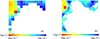 |
Figure 5 Land surface temperature data. (a) Measured data (b) After OK interpolation. |
Background temperature is interpolated using Ordinary Kriging (OK) [26]. OK interpolation, also known as spatial local interpolation, is a method based on semi-variogram theory and structural analysis to provide unbiased optimal estimation of regionalized variables within a finite region. OK interpolation for a single spatial moment is defined as: (9)
(9)
where  (x0) is the value of the location to be predicted; Z(xi) is the actual measured value at the ith location; n is the number of actual measured values in the prediction area; and λi is the weight at the i-th location, the weight [26] can be expressed as:
 (10)where γ(xi,xj) is the variogram between points i and j; γ(xi,x0) is the variogram between point i and point 0 to be estimate; μ is the Lagrange multiplier. When using the OK interpolation method, the sample variogram must first be calculated. Then, an appropriate theoretical model for variogram is selected based on its type for simulation. Finally, a linear estimate of the point to be estimated is performed based on the simulated variogram. The sample variogram [27] is defined as:
![Mathematical equation: $$ \gamma (h)=\frac{1}{2N(h)}={\sum}_{i=1}^{N(h)}{\left[Z\left({x}_i+h\right)-Z\left({x}_i\right)\right]}^2 $$](/articles/jeos/full_html/2026/01/jeos20260006/jeos20260006-eq12.gif) (11)where N(h) is the number of all data pairs with a vector distance of h in the spatial dataset; xi is the coordinate vector of the i-th data point; and h is the vector distance, representing the magnitude and direction of the distance. The spatio-temporal OK interpolation is defined as:
(11)where N(h) is the number of all data pairs with a vector distance of h in the spatial dataset; xi is the coordinate vector of the i-th data point; and h is the vector distance, representing the magnitude and direction of the distance. The spatio-temporal OK interpolation is defined as: (12)where T0(ti) is the OK-predicted baseline temperature at the i-th time instant. Z(xk,ti) is the actual measured temperature at location xk and time ti; λk is the weight assigned to the k-th measured point xk for estimating the value at location x0 and time ti, which is obtained by solving the OK system of equations independently at each time step. The interpolated result is shown in Figure 5b.
2.4.2 Modulation of land surface temperature details
Land surface meteorological data can provide continuous 24-hour temperature variation information and has a high temporal resolution, but its spatial resolution is low, making it difficult to reflect temperature differences at the land surface scale. Therefore, it is necessary to combine meteorological station data with high spatial resolution land surface temperature data retrieved from Landsat 8 to construct a temperature extension model that complements temporal and spatial aspects, in order to achieve a refined spatiotemporal reconstruction of land surface temperature.
Because different land surfaces are located at different altitudes, slopes, and aspects, the atmospheric temperature, humidity, and solar radiation near different land surfaces are different, resulting in subtle fluctuations in temperature. Considering the modulating effect of complex terrain conditions on surface thermal processes, the in-fluence of topographic elevation on surface temperature is introduced in this paper. Key topographic factors such as slope, and aspect are extracted using a digital elevation model (DEM). A multiple linear regression model is constructed to characterize the modulation relationship between topographic parameters and the spatial distribution of surface temperature, thereby achieving a refined simulation of the detailed features of the temperature field.
The slope represents the tilt degree of a certain point on the surface, and the tilt degree of the terrain is measured by calculating the height change of adjacent pixels in two directions. The calculation formula [28] is as follows:![Mathematical equation: $$ Slope\left(x,y\right)=\arctan \left(\sqrt{{\left[\frac{\partial Z}{\partial x}\right]}^2+{\left[\frac{\partial Z}{\partial y}\right]}^2}\right) $$](/articles/jeos/full_html/2026/01/jeos20260006/jeos20260006-eq15.gif) (13)where
(13)where  and
and  denote the elevation gradients in the x and y directions, respectively, which can be approximated by the differences between adjacent pixels. The slope direction represents the slope orientation of a certain point on the surface, and the main direction of the slope is usually calculated [28].
![Mathematical equation: $$ Aspect\left(x,y\right)=\arctan \left(\left[\frac{\partial Z}{\partial y}\right]/\left[\frac{\partial Z}{\partial x}\right]\right) $$](/articles/jeos/full_html/2026/01/jeos20260006/jeos20260006-eq18.gif) (14)The calculation results of slope and aspect are shown in Figures 6a and 6b. Figure 6c shows the elevation data.
(14)The calculation results of slope and aspect are shown in Figures 6a and 6b. Figure 6c shows the elevation data.
 |
Figure 6 Land surface elevation map. (a) Slope calculation results of land surface. (b) Aspect calculation results of land surface. (c) Elevation data. |
The elevation information of the port background has a resolution of 30 m, which is matched with the spatial resolution of the Landsat8 remote sensing image. Multiple DEM raster data are mosaicked and clipped in ArcGIS to obtain the elevation data of the port background area, which is shown in Figure 6. By combining meteorological observation data of the port area to obtain average temperature information of land surface, and based on topographic factors such as slope and aspect, the modulating effect of topography on radiation flux and energy exchange is characterized. A port temperature model is constructed to achieve a re-fined characterization of the temperature field under the combined influence of meteorological conditions and topographic features. (15)where T(x,y,ti) is the predicted temperature at the i-th time instant, Dem(x,y) is the elevation, Slope(x,y) is the slope, Aspect(x,y) is the aspect, T0(ti) is the baseline temperature obtained from meteorological data at the i-th time instant, β1 is the regression coefficient of the elevation factor, the temperature of the land material decreases with the increase of elevation; β2 is the regression coefficient of the slope factor, the slope is negatively correlated with temperature; β3 is the regression coefficient of the aspect factor, the relationship between slope aspect and temperature is “positive in the south and negative in the north”.
The temporal meteorological data is integrated with the spatial background model by pixel-by-pixel. Taking 8:30 in winter as an example, the temperature of the port background is modulated, and the result is shown in Figure 7.
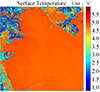 |
Figure 7 The port background temperature after modulated. |
3 Port infrared scene modeling
3.1 Calculation of target temperature distribution
Fluent is widely used in numerical calculation fields such as fluid flow, heat conduction and thermal radiation. It can deal with complex fluid flow and heat transfer process, especially suitable for the simulation of fluid dynamics and heat conduction. The three-dimensional ship target model was established in SpaceClaim. The ship is roughly divided into three components: the deck, hull, and superstructure. Geometric inspection and feature simplification are subsequently performed on the model. Unstructured meshing is then carried out in Workbench Meshing. The global element size is determined based on the overall dimensions of the model, followed by local mesh refinement on key surfaces with significant heat flux variations. The meshing results of the target model are shown in Figure 8.
 |
Figure 8 Ship target grid division diagram. |
The surface temperature of the ship target is solved using Fluent, with the energy equation enabled under steady-state conditions. Turbulence is modeled using the k–ω SST shear stress transfer model [29]. Radiative heat transfer is taken into account through the Discrete Ordinates (DO) model, with solar radiation effects incorporated based on the Solar Ray Tracing algorithm to describe the transmission and distribution of solar energy. The calculation of solar radiation is related to the latitude, and longitude, time zone, date and other factors of port image data. The temperature results in different seasons are shown in Figure 9.
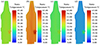 |
Figure 9 Calculation results of ship temperature distribution. (a) Spring. (b) Summer. (c) Autumn. (d) Winter. |
The spatial resolution of the remote sensing background data is 30 m. The ship target calculated in Fluent is modeled at its true scale. In order to match the resolution of the remote sensing image and maintain data consistency, a bilinear interpolation method [30] is adopted to downscale and resample the high-resolution target grid. The coordinates of the known points are (x1, y1), (x1, y2), (x2, y1), (x2, y2). For a given y value, the linear interpolation in the x direction is first performed: (16)
(16) (17)
(17)
Then, interpolation is performed in the y-direction. Substituting the interpolated results obtained in the x-direction into the following equation, the final interpolated value at the target position is obtained: (18)
(18)
In the actual imaging process, when the target completely covers a pixel, the radiation intensity of the pixel is directly determined by the target radiance. When the target does not completely cover a pixel, the radiation intensity of the pixel is the weighted average of the target and the background radiation, and the weight is determined by the area of the target in the pixel.
To verify the accuracy of the calculation model in this paper, the working conditions given in reference [31] are used to reproduce the ship deck temperature using the model in this paper. Four representative typical moments from the literature are selected for simulation, and the average deck temperature at the corresponding moments is calculated. The temperatures calculated in this study are 304.67 K and 280.51 K at 12:00 in summer and winter, respectively, with relative errors of 0.88% and 0.53% compared with the results in reference [31]. At the thermal crossover moment in summer (07:00) and winter (08:00), the temperatures calculated in this paper are 292.08 K and 274.88 K, respectively, with relative errors of 0.72% and 0.04%. The maximum relative error between the calculation results and the measurement data does not exceed 0.88%.
3.2 BRDF modeling of ship target
The Cook-Torrance model is used to calculate the reflected radiation from the ship target surface, taking into account both diffuse and specular reflection occurring on the object’s surface [32]. (19)where kd and ks are the diffuse and specular reflection coefficients of the object surface, respectively; Il is ambient light intensity; F is the Fresnel reflection coefficient; D is the micro-facet distribution function; G is the shading factor; n is the normal direction of the micro-facet; l is the direction vector of the incident light; and v is the observation direction vector. F depends on the properties of the surface material.
4 Modeling of ambient light radiation characteristics
4.1 Modeling of solar radiation characteristics
Solar radiation is the primary energy source for the Earth’s surface, and its intensity and distribution are influenced by latitude, time of day, and atmospheric conditions. In addition, changes in the incident angle and elevation angle of solar radiation, as well as the concentration of suspended particles such as dust and haze in the atmosphere, also play an important role in the intensity and propagation characteristics of radiation. When solar radiation passes through the atmosphere, it is attenuated by substances such as aerosols, clouds, water vapor, and dust, resulting in the absorption or scattering of some of the radiant energy. The solar altitude angle and azimuth angle are calculated based on the local time and the latitude and longitude of the scene [33]. (20)where h is the solar altitude angle; φ is the latitude of the observation point; δ is the solar declination; t is the local time. Using the solar altitude angle and MODTRAN, the incident solar radiation illuminance (Esun) can be calculated. Figure 10 shows the solar incident radiation at different solar altitude angles.
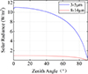 |
Figure 10 The solar incident radiation. |
4.2 Modeling of sky radiation characteristics
Sky radiation is the scattered radiation of solar radiation. The sky background radiation is regarded as a hemispherical space that emits radiation outward. The sky radiation incident from different directions can be calculated using MODTRAN [28]. Figure 11 shows the sky incident radiation at different wavelengths.
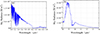 |
Figure 11 The sky incident radiation. |
4.3 Modeling of atmospheric radiation characteristics
The atmospheric attenuation effect has a significant impact on the upward radiative transmission of the target and background. The atmosphere itself will generate infrared radiation. The total atmospheric path radiation in the detection direction [34] is shown:![Mathematical equation: $$ {L}_a\left(\lambda \right)={\int}_0^r{L}_{\lambda}\left({r}^{\prime}\right)\exp \left[{\tau}^{\prime}\left({r}^{\prime}\right)-{\tau}^{\prime }(r)\right]{dr}^{\prime } $$](/articles/jeos/full_html/2026/01/jeos20260006/jeos20260006-eq27.gif) (21)where r is the distance between the target and the observation point; L(r′) is the spectral radiance of the path point; τ’ is the atmospheric path optical depth.
(21)where r is the distance between the target and the observation point; L(r′) is the spectral radiance of the path point; τ’ is the atmospheric path optical depth.
Meanwhile, aerosol particles and molecules in the atmosphere have absorption and scattering effects on the upward radiation of the target and background, resulting in the attenuation of the target and background radiation. The atmospheric attenuation capacity of a target varies under different meteorological conditions. Atmospheric spectral transmittance is generally used to describe the degree of atmospheric attenuation. Once the scene geometry is determined, atmospheric path radiation and atmospheric transmittance can be calculated using MODTRAN. The atmospheric parameters are configured as follows: atmospheric condition is mid-latitude summer, aerosol model is naval ocean, weather conditions are cloudless and rainless, and visibility is 23 km. The calculation results are presented in Figure 12.
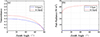 |
Figure 12 Atmospheric radiation characteristics calculation result. |
Meanwhile, the atmospheric conditions are chosen to be mid-latitude winter to calculate the atmospheric radiation transfer characteristics under winter conditions. The calculation results are shown in Figure 13.
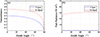 |
Figure 13 Atmospheric radiation characteristics calculation result. |
5 Results
5.1 3–5 μm simulation results
The simulation parameters are selected as follows: focal length is 1.06 m, optical system transmittance is 0.7, aperture is 0.53 m, pixel size is 40 μm, and orbital altitude is 795 km, emissivity of the hull, deck and superstructure is 0.85, 0.90, 0.78, respectively. In target detection research, the signal-to-clutter ratio (SCR) has significant advantages as an evaluation metric. The SCR [18] can quantitatively characterize the distinguishability of a target’s radiated relative to background clutter, reflecting the target’s detectability under complex background conditions. (22)where SCR is the local signal-to-clutter ratio; Ītrg is the average radiation luminance of the target; Ībg is the mean background value within an area twice the size of the target; σb is the background variance within an area twice the size of the target. Figure 14 shows the simulation results of the infrared imaging characteristics of ship targets at different times in 3–5 μm band. Figure 15 shows the SCR in the 3–5 μm band.
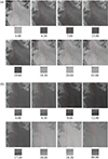 |
Figure 14 Simulation results of ship infrared imaging features of 3–5 μm. (a) Typical time in Summer. (b) Typical time in Winter. |
 |
Figure 15 SCR in the 3–5 μm band. (a) Summer. (b) Winter. |
As can be seen from Figures 14 and 15, the radiation values of the target and background change dynamically throughout the day. Due to seasonal differences, the target radiation value generally higher in summer than in winter. The difference in radiation between the target and background is greatest at 13:00 and 01:00 in summer, resulting in higher SCR values, making the target most easily detectable at these times. Due to the lack of solar radiation at night, the target radiation is generally lower than the background radiation, appearing as a dark target at 6:00. As solar radiation gradually increases after sunrise, the target temperature rises rapidly. During the period from 6:00 to 6:30, the difference between the target and the background radiation gradually decreases, and at 6:30, the radiation of the target and the background reaches a state of approximately equality, which is the zero-crossing moment of thermal equilibrium. At this time, the contrast between the target and the background is extremely low, and the target is almost submerged by background clutter, which is a typical thermal crossover stage. Subsequently, between 6:30 and 7:00, the target radiation continues to increase and gradually exceeds the background. At 7:00, the radiation contrast between the target and the background reverses, and the target changed from dark to bright. Between 19:00 and 20:00, the radiation difference between the target and the background undergoes another reversal of the contrast relationship. At 19:30, the target is in a typical thermal crossover state, where the radiation intensity of the target and the background are approximately equal and the contrast is significantly reduced. After that, the target radiation further decreases and falls below the background radiation, and the target changes from a bright target to a dark target.
In winter, the local SCR is large at 12:00 and 00:00, and the target is more detectable. However, the target radiation is larger than the background at 12:00, and the opposite is true at 00:00. The critical points for “thermal crossover” occur around 8:30 and 18:30. Therefore, it can be seen that in the 3–5 μm band, at the critical moment of thermal crossover, the detectability is better in winter than in summer; while in non-thermal crossover periods, the opposite is true.
5.2 8–14 μm simulation results
Figure 16 shows the simulation results of the infrared optical imaging characteristics of ship targets at different times in the 8–14 μm band. Emissivity of the hull, deck and superstructure is 0.90, 0.95, 0.88, respectively. The local SCR in the 8–14 μm band is calculated, and the results are shown in Figure 16.
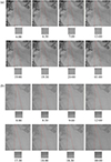 |
Figure 16 Simulation results of ship infrared imaging features of 8–14 μm. (a) Typical time of Summer. (b) Typical time of Winter. |
Combining Figures 16 and 17, it can be seen that in summer, the local SCR is the highest at 01:00, and the target detection capability is the strongest, but the target radiation intensity is lower than the background. At 13:00, the target radiation intensity is higher than the background, indicating that the target is detectable. At the other two moments, due to changes in ambient temperature, the background and target radiation characteristics are similar, and the target difficult to detect.
 |
Figure 17 SCR in the 8–14 μm band. (a) Summer. (b) Winter. |
In winter, the local SCR is relatively large at 12:00 and 00:00, and the target detection capability is relatively strong. The critical point of “thermal crossover” appears around 8:30 and 18:00. In the 8–14 μm band, during the critical moment of thermal crossover, the detectability is better in summer than in winter; during non-thermal crossover periods, the opposite is true.
Comparing Figures 14 and 16, it can be seen that the occurrence of the thermal crossover phenomenon in the morning happens earlier in summer than in winter, while the thermal crossover time in the evening occurs later in summer than in winter. This phenomenon is caused by the varying solar radiation in different seasons and differences in the heat absorption characteristics of materials. Comparing Figures 15 and 17, it can be seen that the evolution of ship imaging characteristics at the critical moment of “thermal crossover” is correlated with both season and time. During non-thermal crossover periods in summer, the detectability of 3–5 μm is better than that of 8–14 μm, while the opposite is true during non-thermal crossover periods in winter. During the critical moment of thermal crossover in summer, the detectability of 3–5 μm is worse than that of 8–14 μm, while during the critical moment of thermal crossover in winter, the detectability of 3–5 μm and 8–14 μm is relatively close.
At the thermal crossover moment, the thermal radiation difference between the target and the background is relatively small, and the radiative signal is mainly constrained by atmospheric transmittance and path radiance. In summer, atmospheric humidity and temperature are higher than in winter, causing the target radiative characteristics in the 3–5 μm band to be significantly affected by water vapor absorption and atmospheric thermal radiation interference, whereas the 8–14 μm band is less influenced by atmospheric radiative transfer, resulting in less pronounced variations in target radiative characteristics. In winter, atmospheric humidity and temperature are low, the difference in atmospheric radiation between the two bands decreases, and the target radiation characteristics tend to converge.
6 Conclusion
To address the limitation of infrared detection systems in detecting surface ships during “thermal crossover” periods, an optical imaging feature prediction model of ship target, port background, ambient lighting, and atmosphere is established. The imaging characteristics during thermal crossover periods of ship targets in the 3–5 μm and 8–14 μm bands are simulated and analyzed. The detectability of low-orbit satellites to ship targets under different environmental conditions is analyzed using local SCR. The results show that the radiation difference between the target and the background exhibits a clear stage-wise evolution before and after the thermal crossover. As the background temperature gradually approaches the target temperature, the radiation contrast of the target in infrared imaging decreases significantly, which means that the target’s detectability weakens over time. Near the moment of thermal crossover, the contrast between the target and the background reaches its lowest value, which will have a significant impact on the detection algorithm and recognition performance. Meanwhile, the sensitivity to thermal crossover varies across different bands, indicating that appropriate band selection is of great significance for target detection. The results will provide data support and theoretical basis for the infrared detection and identification of ship targets in complex marine environments.
Funding
Shaanxi Provincial Natural Science Basic Research Program Project (2025JC-YBQN-845, 2025JC-YBQN-081); Shaanxi Province Postdoctoral Research Project (2023BSHEDZZ161).
Author contribution statement
Conceptualization, HANG YUAN and JIAHUI REN; methodology, HANG YUAN; software, JIAHUI REN; validation, YANG ZHANG, HANG YUAN and JIAHAO MIN; formal analysis, HANG YUAN; resources, HANG YUAN; data curation, HANG YUAN; writing-original draft preparation, HANG YUAN and JIAHUI REN; writing-review and editing, HANG YUAN and JIAHUI REN; visualization, JIAHUI REN and JIAHAO MIN; supervision, HANG YUAN; project administration, HANG YUAN; funding acquisition, HANG YUAN and ZHENG ZHANG. All authors have read and agreed to the published version of the manuscript.
Conflicts of interest
The authors declare no conflicts of interest.
Data availability statement
Data associated with this article are available from the corresponding author upon reasonable request.
References
- Chen X, Qiu C, Zhang Z, A multiscale method for infrared ship detection based on morphological reconstruction and two-branch compensation strategy, Sensors 23, 7309 (2023). https://doi.org/10.3390/s23167309. [Google Scholar]
- Song W et al., Ship detection and identification in SDGSAT-1 glimmer images based on the glimmer YOLO model, Int, J. Digital Earth 16(2), 4687–4706 (2023).https://doi.org/10.1080/17538947.2023.2277796. [Google Scholar]
- Kim DG et al., Comparison of measured and simulated IR signals from a scaled model ship, Proc. Spie 8857, 438–445 (2013). https://doi.org/10.1117/12.2024155. [Google Scholar]
- Bin C et al., Infrared simulation research based on warships and ocean wake background, Comp. Dig. Eng. 42(7), 1248–1250 (2014).http://doi.org/10.3969/j.issn1672-9722.2014.07.032. [Google Scholar]
- Lin J et al., Infrared radiation characteristics simulation of exhaust suppression type ships, Infrared Phys. Technol. 141, 105499 (2024). https://doi.org/10.1016/j.infrared.2024.105499. [Google Scholar]
- Jiang Z et al., Simulation method for infrared radiation transmission characteristics of typical ship targets based on optical remote sensing, Concurrency Computat. Pract. Exper., e7515 (2022). https://doi.org/10.1002/cpe.7515. [Google Scholar]
- Zhang CW et al., Electromagnetic scattering and imaging simulation of extremely large-scale sea-ship scene based on GPU parallel technology, J. Electron Sci. Technol. 22(2), 16–23 (2024https://doi.org/10.1016/j.jnlest.2024.100257. [Google Scholar]
- Wang M et al., Research on modeling methods of infrared radiation characteristics of sea surface targets, AOPC 2024: Infrared Technology and Applications. Proc. Spie 13493, 84–92 (2024).https://doi.org/10.1117/12.3047745. [Google Scholar]
- Bo S et al., Simulation method of high resolution satellite imaging for sea surface target, Infrared Laser Eng. 50(12), 20210127 (2021https://doi.org/10.3788/IRLA20210127 [Google Scholar]
- Jiang L et al., Near infrared scene simulation based on reflectance of typical target, Acta Photonica Sinica, 43(8), 132–137 (2014). https://doi.org/10.3788/gzxb20144308.0810004. [Google Scholar]
- Wang X et al., Multi – band infrared radiation characterization and simulation analysis for aerial target, Acta Photonica Sinica 49(5), 110–120 (2020). http://doi.org/10.3788/gzxb20204905.0511002. [Google Scholar]
- Laleh R E, Ghasemloo N, Calculate thermal infrared intensity of the hull’s military ship, J. Geogr. Inf. Syst. 6(4), 317–329 (2014). http://doi.org/10.4236/jgis.2014.64029. [Google Scholar]
- Llorente SDPM, Charris VD, Torres JMG, Infrared signature analysis of surface ships, Ciencia y tecnología de buques 8(17), 57–68 (2015). https://doi.org/10.25043/19098642.121. [Google Scholar]
- Sun W et al., Digital imaging simulation and closed-loop verification model of infrared payloads in space-based cloud–sea scenarios, Remote Sens. 17(16), 2900 (2025). https://doi.org/10.3390/rs17162900. [Google Scholar]
- Li M et al., Infrared image generation method based on visible images and its detail modulation, Inf. Technol. 40, 34–38 (2018). https://link.cnki.net/urlid/53.1053.TN.20180131.1321.014 [Google Scholar]
- Yuan H et al., Space-based full chain multi-spectral imaging features accurate prediction and analysis for aircraft plume under sea/cloud background, Opt. Express 27(18), 26027–26043 (2019). https://doi.org/10.1364/oe.27.026027. [Google Scholar]
- Yuan H et al., Performance analysis of the infrared imaging system for aircraft plume detection from geostationary orbit, Appl. Opt 58(7), 1691–1698 (2019). https://doi.org/10.1364/AO.58.001691. [Google Scholar]
- Xie C et al., Prediction and simulation analysis of infrared polarization imaging characteristics of aerodynamic heating targets in orbit under sea background, Infrared Laser Eng. 53(11), 20240222 (2024). http://doi.org/10.3788/IRLA20240222. [Google Scholar]
- Bai Y et al., Occlusion and deformation handling visual tracking for UAV via attention-based mask generative network, Remote Sens. 14, 4756 (2022). https://doi.org/10.3390/rs14194756. [Google Scholar]
- Wang P et al., Traffic thermal infrared texture generation based on siamese semantic CycleGAN, Infrared Phys. Technol. 116, 103748 (2021). https://doi.org/10.1016/j.infrared.2021.103748. [Google Scholar]
- Pan M et al., Infrared image generation technique based on GAN network, Flight Control Detect. 4, 1–6 (2021). http://doi.org/10.20249/j.cnki.2096-5974.2021.04.001. [Google Scholar]
- Liang X, Meng Q, Wang C, Infrared thermal image simulation of ships at sea in the long-wave band, Appl. Opt. 46(4), 877–885 (2025). http://doi.org/10.5768/JAO202546.0404001. [Google Scholar]
- Li H et al., Hsiao framework in feature selection for hyperspectral remote sensing images based on jeffries-matusita distance, IEEE Trans. Geosci. Remote Sens. 63,1–21 (2025). https://doi.org/10.1109/TGRS.2025.3527138. [Google Scholar]
- Vanhelmont Q, Combined land surface emissivity and temperature estimation from Landsat 8 OLI and TIRS, ISPRS J. Photogramm. Remote Sens. 166, 390–402 (2020). https://doi.org/10.1016/j.isprsjprs.2020.06.007. [Google Scholar]
- Yang XF, Ye M, Mao DL, Application of BRDF model in land cover mapping, J. East China normal Univ. (Nat. Sci.) 01, 113–124 (2017). https://doi.org/10.3969/j.issn.1000-5641.2017.01.013. [Google Scholar]
- Wand YP et al., Evaluation and analysis of effects on the different interpolation temperature algorithms, Inf. Technol. 44(6), 31–35 (2020). http://doi.org/10.13274/j.cnki.hdzj.2020.06.008. [Google Scholar]
- Liu Y et al., A non-uniform spatiotemporal kriging interpolation algorithm for landslide displacement data. Bulletin of Engineering Geology and the Environment, 78(6), 4153–4166 (2019).https://doi.org/10.1007/s10064-018-1388-1. [Google Scholar]
- Long Y Q et al., Difference analysis of slope extraction from DEM based on different directional reference systems, J. Mt. Sci. 36(3), 462–469 (2018). https://doi.org/10.16089/j.cnki.1008-2786.000342. [Google Scholar]
- Banker ND, Numerical investigation of heat transfer in aircraft engine blade using k ∈ and SST k ω model, IOP Conference Series: Materials Science and Engineering 1013(1), 012027 (5pp) (2021). https://doi.org/10.1088/1757-899X/1013/1/012027. [Google Scholar]
- Huang Y, Liao X, Lu Q, Infrared image interpolation algorithm based on bilinear interpolation and local mean, Comput. Technol. Autom. 39(2), 133–137 (2020). http://doi.org/10.16339/j.cnki.jsjsyzdh.202002027. [Google Scholar]
- Zhang L, Qiao K, Huang S, Spectrum selection and performance analysis for ship detection, J. Infrared Millim. Waves 43(2), 234–240 (2024). https://doi.org/10.11972/j.issn.1001-9014.2024.02.013. [Google Scholar]
- Wang X, Gao SL, Li FM, Infrared imaging modeling and simulation of aerial targets based on BRDF, J. Infrared Milliwave 38(2), 182–187 (2019). http://doi.org/10.11972/j.issn.1001-9014.2019.02.010. [Google Scholar]
- Alonso S et al., A solar altitude angle model for efficient solar energy predictions, Sensors 20(5), 1391 (2020). https://doi.org/10.3390/s20051391. [Google Scholar]
- Huang Z L et al., Infrared simulation imaging of ship wakes and sea surface, J. Appl. Opt. 44(2), 286–294 (2023https://doi.org/10.5768/JAO202344.0201007. [Google Scholar]
All Tables
All Figures
|
Figure 1 Space-based optoelectronic system detecting targets. |
| In the text | |
|
Figure 2 The temperature distribution of the four seasons in the port. (a) Spring. (b) Summer. (c) Autumn. (d) Winter. |
| In the text | |
|
Figure 3 The supervised classification process. |
| In the text | |
|
Figure 4 Land surface classification result. |
| In the text | |
|
Figure 5 Land surface temperature data. (a) Measured data (b) After OK interpolation. |
| In the text | |
|
Figure 6 Land surface elevation map. (a) Slope calculation results of land surface. (b) Aspect calculation results of land surface. (c) Elevation data. |
| In the text | |
|
Figure 7 The port background temperature after modulated. |
| In the text | |
|
Figure 8 Ship target grid division diagram. |
| In the text | |
|
Figure 9 Calculation results of ship temperature distribution. (a) Spring. (b) Summer. (c) Autumn. (d) Winter. |
| In the text | |
|
Figure 10 The solar incident radiation. |
| In the text | |
|
Figure 11 The sky incident radiation. |
| In the text | |
|
Figure 12 Atmospheric radiation characteristics calculation result. |
| In the text | |
|
Figure 13 Atmospheric radiation characteristics calculation result. |
| In the text | |
|
Figure 14 Simulation results of ship infrared imaging features of 3–5 μm. (a) Typical time in Summer. (b) Typical time in Winter. |
| In the text | |
|
Figure 15 SCR in the 3–5 μm band. (a) Summer. (b) Winter. |
| In the text | |
|
Figure 16 Simulation results of ship infrared imaging features of 8–14 μm. (a) Typical time of Summer. (b) Typical time of Winter. |
| In the text | |
|
Figure 17 SCR in the 8–14 μm band. (a) Summer. (b) Winter. |
| In the text | |
Current usage metrics show cumulative count of Article Views (full-text article views including HTML views, PDF and ePub downloads, according to the available data) and Abstracts Views on Vision4Press platform.
Data correspond to usage on the plateform after 2015. The current usage metrics is available 48-96 hours after online publication and is updated daily on week days.
Initial download of the metrics may take a while.