© The Author(s), published by EDP Sciences, 2026

1 Introduction

Zernike polynomials play a key role in many optical applications [1–3] due to their two main features: 1. the orthogonality between individual polynomial components and 2. the direct correspondence with optical Seidel aberrations. Zernike polynomials are usually defined as$$z_n^{\pm m}(\rho ,\phi )=R_n^m\left(\rho \right)\{\begin{array}{ccc}\cos \left(\mathrm{m\phi }\right)& \mathrm{for} & +m\\ \sin \left(\mathrm{m\phi }\right)& \mathrm{for} & -m\end{array},$$(1) $$R_n^m=\sum _{k=0}^{(n-m)/2}\left(\frac{(-1{)}^k(n-k)!}{k!\left(\frac{n+m}{2}-k\right)!\left(\frac{n-m}{2}-k\right)!}{\rho }^{n-2k}\right),$$(2)

where $R_n^m$ is called the Zernike radial polynomial. The above equations appear in the literature [4, 5] with different notations for the m-term. This work adopts the ±m notation since this notation provides an explicit and convenient way to divide Zernike components of order n into their even part (±m = ±2l), and their odd part ±m = ± (2l + 1), and to subdivide each part into distinct cos and sin subparts. Incidentally, all odd parts of the components for the even order (n = 2j) and all even parts of the components for the odd order (n = 2j + 1) are discarded to avoid non-integer factorials in Zernike radial polynomials (Eq. (2)), and all index terms n, m, l, j, k in this work are non-negative integers, and l ≤ j and k ≤ (j − l).

If the polynomial order is not high, the calculation of Zernike polynomials is usually satisfied by the definition formulas. For Zernike radial polynomials a three-term-recurrence-relation (TTRR) exists and has been applied component-wise to higher-order recursive Zernike calculations [6, 7]:$$R_n^m=\rho \left(R_{n-1}^{|m-1|}\left(\rho \right)+R_{n-1}^{m+1}\left(\rho \right)\right)-R_{n-2}^m\left(\rho \right).$$(3)

On the other hand, Zernike polynomials are essentially one of the orthogonalized versions of the homogeneous bivariate polynomials in a Cartesian coordinate system with a unit circle and a coordinate center. In practice, the computation of Zernike polynomials is often based on a look-up-table (LUT) of the corresponding Cartesian forms of the individual Zernike components [3, 8, 9], although the complexity of such Cartesian forms increases sharply with polynomial order.

To achieve greater flexibility compared to component-wise recursive computations, and to lower the limits of polynomial order and complexity in Cartesian form based computations, this work uncovers two cases of block-wise recurrence in Zernike computations¹ and offers both a direct block-wise transformation method and a block-wise recursive method for matrix-form Zernike computations. The application of such block-wise methods promises higher computational speed and lower memory footprint without compromising accuracy.

The rest of this paper is organized as follows: The next section presents two hidden block-wise recurrences along with their close relationship to an n-row Pascal’s triangle; subsequently Section 3 explores a new computation scheme for Zernike polynomials, which covers basis function computation, coefficient determination, polar/Cartesian coordinate conversion, and application specific derivative analysis, among others; further technical discussions can be found in Section 4, where a preliminary performance evaluation is conducted in term of computational complexity, accuracy stability, memory requirements, and application flexibility; finally, Section 5 concludes this paper with an outlook on future works.

2 Zernike polynomials supported by one Pascal’s triangle

2.1 Pascal triangle supported block-wise recurrence

The Zernike radial polynomials of the first n ≤ 6 orders can be expressed in matrix form, where all radial polynomials of an order are obtained by multiplying a coordinate value irrelevant factor matrix by a power vector of the radial coordinate values, as:$$\{\begin{array}{ll}{R}_0^0\left(\rho \right)& =1\\ R_1^1\left(\rho \right)& =\rho \\ R_2^0\left(\rho \right)& =2{\rho }^2-1\\ R_2^2\left(\rho \right)& ={\rho }^2\\ R_3^1\left(\rho \right)& =3{\rho }^3-2\rho \\ R_3^3\left(\rho \right)& ={\rho }^3\\ R_4^0\left(\rho \right)& =6{\rho }^4-6{\rho }^2+1\\ R_4^2\left(\rho \right)& =4{\rho }^4-3{\rho }^2\\ R_4^4\left(\rho \right)& ={\rho }^4\\ R_5^1\left(\rho \right)& =10{\rho }^5-12{\rho }^3+3\rho \\ R_5^3\left(\rho \right)& =5{\rho }^5-4{\rho }^3\\ R_5^5\left(\rho \right)& ={\rho }^5\\ R_6^0\left(\rho \right)& =20{\rho }^6-30{\rho }^4+12{\rho }^2-1\\ R_6^2\left(\rho \right)& =15{\rho }^6-20{\rho }^4+6{\rho }^2\\ R_6^4\left(\rho \right)& =6{\rho }^6-5{\rho }^4\\ R_6^6\left(\rho \right)& ={\rho }^6\end{array}⟹\{\begin{array}{ll}{R}_0^{\left\{m\right\}}& =1\times {\rho }^0\\ R_1^{\left\{m\right\}}& =1\times {\rho }^1\\ R_2^{\left\{m\right\}}& =\left[\begin{array}{ll}2& -1\\ 1& 0\end{array}\right]\times \left[\begin{array}{l}{\rho }^2\\ {\rho }^0\end{array}\right]\\ R_3^{\left\{m\right\}}& =\left[\begin{array}{ll}3& -2\\ 1& 0\end{array}\right]\times \left[\begin{array}{l}{\rho }^3\\ {\rho }^1\end{array}\right]\\ R_4^{\left\{m\right\}}& =\left[\begin{array}{lll}6& -6& 1\\ 4& -3& 0\\ 1& 0& 0\end{array}\right]\times \left[\begin{array}{l}{\rho }^4\\ {\rho }^2\\ {\rho }^0\end{array}\right]\\ R_5^{\left\{m\right\}}& =\left[\begin{array}{lll}10& -12& 3\\ 5& -4& 0\\ 1& 0& 0\end{array}\right]\times \left[\begin{array}{l}{\rho }^5\\ {\rho }^3\\ {\rho }^1\end{array}\right]\\ R_6^{\left\{m\right\}}& =\left[\begin{array}{llll}20& -30& 12& -1\\ 15& -20& 6& 0\\ 6& -5& 0& 0\\ 1& 0& 0& 0\end{array}\right]\times \left[\begin{array}{l}{\rho }^6\\ {\rho }^4\\ {\rho }^2\\ {\rho }^0\end{array}\right]\end{array}$$(4)

where $R_n^{\left\{m\right\}}$ denotes a column vector ${\left[\begin{array}{llll}{R}_{2j}^0& R_{2j}^2& \cdots & R_{2j}^{2j}\end{array}\right]}^T$ for even orders (n = 2j) or ${\left[\begin{array}{llll}{R}_{2j+1}^1& R_{2j+1}^3& \cdots & R_{2j+1}^{2j+1}\end{array}\right]}^T$ for odd orders (n = 2j + 1).

From the above equation seven weight vectors, $\{w_n^{\left\{k\right\}} |n=\mathrm{0,1},...,6\}$ with 0 ≤ k ≤ j, can be extracted from the corresponding order-specific factor matrices (Eq. (5)). A block-wise recurrence among the de-weighted factor matrices ({T _n |n = 0, 1, …, 6}) can be observed: the 0th order de-weighted factor matrix appears in the 2nd order de-weighted factor matrix, while the later subsequentially appears in the 4th order de-weighted factor matrix, which in turn appears in the 6th order de-weighted factor matrix. The same applies to odd orders from the 1st order to the 5th order, as follows:$$\{\begin{array}{ll}{R}_0^{\left\{m\right\}}& =1\times \mathrm{diag}\left(1\right)\times {\rho }^0\\ R_1^{\left\{m\right\}}& =1\times \mathrm{diag}\left(1\right)\times {\rho }^1\\ R_2^{\left\{m\right\}}& =\left[\begin{array}{ll}2& 1\\ 1& 0\end{array}\right]\times \mathrm{diag}\left({\left[\begin{array}{l}1\\ -1\end{array}\right]}^T\right)\times \left[\begin{array}{l}{\rho }^2\\ {\rho }^0\end{array}\right]\\ R_3^{\left\{m\right\}}& =\left[\begin{array}{ll}3& 1\\ 1& 0\end{array}\right]\times \mathrm{diag}\left({\left[\begin{array}{l}1\\ -2\end{array}\right]}^T\right)\times \left[\begin{array}{l}{\rho }^3\\ {\rho }^1\end{array}\right]\\ R_4^{\left\{m\right\}}& =\left[\begin{array}{lll}6& 2& 1\\ 4& 1& 0\\ 1& 0& 0\end{array}\right]\times \mathrm{diag}\left({\left[\begin{array}{l}1\\ -3\\ 1\end{array}\right]}^T\right)\times \left[\begin{array}{l}{\rho }^4\\ {\rho }^2\\ {\rho }^0\end{array}\right]\\ R_5^{\left\{m\right\}}& =\left[\begin{array}{lll}10& 3& 1\\ 5& 1& 0\\ 1& 0& 0\end{array}\right]\times \mathrm{diag}\left({\left[\begin{array}{l}1\\ -4\\ 3\end{array}\right]}^T\right)\times \left[\begin{array}{l}{\rho }^5\\ {\rho }^3\\ {\rho }^1\end{array}\right]\\ R_6^{\left\{m\right\}}& =\left[\begin{array}{llll}20& 6& 2& 1\\ 15& 4& 1& 0\\ 6& 1& 0& 0\\ 1& 0& 0& 0\end{array}\right]\times \mathrm{diag}\left({\left[\begin{array}{l}1\\ -5\\ 6\\ -1\end{array}\right]}^T\right)\times \left[\begin{array}{l}{\rho }^6\\ {\rho }^4\\ {\rho }^2\\ {\rho }^0\end{array}\right]\end{array}⟹R_{n\le 6}^{\left\{m\right\}}=T_n\times \mathrm{diag}\left(w_n^{\left\{k\right\}}\right)\times \left[\begin{array}{l}{\rho }^n\\ {\rho }^{n-2}\\ ⋮\\ {\rho }^{\left(n\mathrm{mod}2\right)}\end{array}\right],$$(5)

where $\mathrm{diag}\left(w_n^{\left\{k\right\}}\right)$ denotes the diagonalization of a vector to a diagonal matrix, as$$\mathrm{diag}\left(w_n^{\left\{k\right\}}\right)=\left[\begin{array}{llll}{w}_n^0& 0& \cdots & 0\\ 0& w_n^1& \cdots & 0\\ ⋮& ⋮& \ddots & ⋮\\ 0& 0& \cdots & w_n^j\end{array}\right].$$(6)

It appears that for order n ≥ 2, the de-weighted factor matrix T _n can be interpreted as an extended T _n−2, with zero-padding at the bottom and a factor vector $t_n^{\left\{m\right\}}$ attached to its left side, as described in the following equation:$$\{\begin{array}{ll}{T}_0& =1\\ T_1& =1\\ T_{n\le 6}& =\left[\begin{array}{ll}{t}_n^{\left\{m\right\}}& \left[\begin{array}{l}{T}_{n-2}\\ 0\end{array}\right]\end{array}\right]\end{array}.$$(7)

Note that both the extracted weight vector $w_n^{\left\{k\right\}}$ and the de-weighted factor vector $t_n^{\left\{m\right\}}$ are closely related to an n-row Pascal triangle. In particular, $t_n^{\left\{m\right\}}$ corresponds to the right half of the nth row vector in a standard Pascal triangle (Table 1), i.e., here we have $t_6^{\left\{m\right\}}=[\begin{array}{llll}20& 15& 6& 1\end{array}{]}^T$, $t_5^{\left\{m\right\}}=[\begin{array}{lll}10& 5& 1\end{array}{]}^T$, $t_4^{\left\{m\right\}}=[\begin{array}{lll}6& 4& 1\end{array}{]}^T$, $t_3^{\left\{m\right\}}=[\begin{array}{ll}3& 1\end{array}{]}^T$, $t_2^{\left\{m\right\}}=[\begin{array}{ll}2& 1\end{array}{]}^T$, $t_1^{\left\{m\right\}}=1$ and $t_0^{\left\{m\right\}}=1$ for radial polynomials of orders n ≤ 6; On the other hand, all extracted weight vectors $w_n^{\left\{k\right\}}$ can be found as corresponding anti-diagonal vectors in the left-aligned Pascal triangle (Table 2), as $w_{\mathrm{0,1}}^{\left\{k\right\}}=1$, $w_2^{\left\{k\right\}}=\left[\begin{array}{ll}1& -1\end{array}\right]$, $w_3^{\left\{k\right\}}=\left[\begin{array}{ll}1& -2\end{array}\right]$, $w_4^{\left\{k\right\}}=\left[\begin{array}{lll}1& -3& 1\end{array}\right]$, $w_5^{\left\{k\right\}}=\left[\begin{array}{lll}1& -4& 3\end{array}\right]$, $w_6^{\left\{k\right\}}=\left[\begin{array}{llll}1& -5& 6& -1\end{array}\right]$, where all odd elements (numbered from 0 onwards) are additionally assigned a negative sign.

To our knowledge, the above-mentioned discoveries are rarely discussed in the literature. Therefore, it is necessary to prove that these discoveries, i.e., the separation of coordinate-relevant and -irrelevant computations (Eq. (4)), the extraction of order-specific weight vectors (Eq. (5)), the block-wise recurrence within de-weighted factor matrices (Eq. (7)), and the close relationship to an n-row Pascal triangle (Tables 1 and 2), hold for Zernike radial polynomials without order limit (i.e., ∀n > 6); if possible and expected, this also holds for complete Zernike polynomials (i.e., radial × azimuth polynomials).

2.2 From canonical to block-wise Zernike calculation

The canonical definition of Zernike radial polynomials, equation (2), has its binomial form:$$R_n^m=\sum _{k=0}^{(n-m)/2}(-1{)}^k\left(\begin{array}{l}n-k\\ k\end{array}\right)\left(\begin{array}{l}n-2k\\ \frac{n-m}{2}-k\end{array}\right){\rho }^{n-2k}.$$(8)

If we swap the terms m and k in the second binomial term, we obtain$$R_n^m=\sum _{k=0}^{(n-m)/2}(-1{)}^k\left(\begin{array}{l}n-k\\ k\end{array}\right)\left(\begin{array}{l}n-2k\\ \frac{n-2k}{2}-\frac{m}{2}\end{array}\right){\rho }^{n-2k}.$$(9)

In this equation, the term $\left(\begin{array}{l}n-k\\ k\end{array}\right)$ explicitly denotes the anti-diagonal vectors in a left-aligned Pascal triangle, and the term $\left(\begin{array}{l}n-2k\\ \frac{n-2k}{2}-\frac{m}{2}\end{array}\right)$ denotes the left and right halves of the (n − 2k)th-row in a standard Pascal triangle, since Pascal’s triangle has its mirror symmetry with respect to its center position $\frac{n-2k}{2}$.

By Combining de Moivre’s formula (cosmφ + isinmφ) = (cosφ + isinφ)^m with the radial polynomials and converting the coordinate system from polar to Cartesian coordinates, we obtain a direct block-wise transformation method for calculating Zernike basis functions in the Cartesian coordinate system. If we define $X_j^{\left\{q\right\}}={\left[\begin{array}{llll}{x}^{2j}{y}^0& x^{2j-2}{y}^2& \cdots & x^0{y}^{2j}\end{array}\right]}^T$, and set $w_n^k=(-1{)}^k\left(\begin{array}{l}n-k\\ k\end{array}\right)$ and $t_n^{\{l=m/2\}}=\left(\begin{array}{l}n-2k\\ \frac{n-2k}{2}-\frac{\left\{m\right\}}{2}\end{array}\right)$, where {l} denotes the index vector as $\left\{l\right\}=[\begin{array}{llll}0& 1& \cdots & n/2\end{array}{]}^T$ for even orders or $\left\{l\right\}=[\begin{array}{llll}0& 1& \cdots & (n-1)/2\end{array}{]}^T$ for odd orders, then such a direct block-wise transformation is represented as a transformation of homogeneous bivariate (xy) polynomials into complete Zernike polynomials, as the following:$$\{\begin{array}{ll}{z}_{2j}^{-\left\{2l\right\}}=& \sum _{k=0}^j\mathrm{}{w}_{2j}^k\left(t_{2(j-k)}^{\left\{l\right\}}\odot B_{2(j-k)}^{-}\right)\times X_{(j-k)}^{\left\{q\right\}}{x}^{-1}y\\ z_{2j}^{+\left\{2l\right\}}=& \sum _{k=0}^j\mathrm{}{w}_{2j}^k\left(t_{2(j-k)}^{\left\{l\right\}}\odot B_{2(j-k)}^{+}\right)\times X_{(j-k)}^{\left\{q\right\}}\\ z_{2j+1}^{-\{2l+1\}}=& \sum _{k=0}^j\mathrm{}{w}_{2j+1}^k\left(t_{2(j-k)+1}^{\left\{l\right\}}\odot B_{2(j-k)+1}^{-}\right)\times X_{(j-k)}^{\left\{q\right\}}y\\ z_{2j+1}^{+\{2l+1\}}=& \sum _{k=0}^j\mathrm{}{w}_{2j+1}^k\left(t_{2(j-k)+1}^{\left\{l\right\}}\odot B_{2(j-k)+1}^{+}\right)\times X_{(j-k)}^{\left\{q\right\}}x\\ & \end{array},$$(10)

where the terms of $B_{2j}^{-},B_{2j}^{+},B_{2j+1}^{-}$ and $B_{2j+1}^{+}$ denote four coordinate transformation matrices from the polar coordinate system to the Cartesian coordinate system for corresponding cos/sin components in Zernike basis functions of even and odd order. These four transformation matrices form the second block-wise recurrence in Zernike computations, since the following recursion relation holds: ² $$\{\begin{array}{ll}{B}_0^{-}& =0,B_0^{+}=1,B_1^{-}=1,B_1^{+}=1\\ B_{2j}^{-}& =\left[\begin{array}{ll}0& 0\\ B_{2j-1}^{+}+B_{2j-1}^{-}& 0\end{array}\right]\\ B_{2j}^{+}& =\left[\begin{array}{l}\left[\begin{array}{ll}{B}_{2j-1}^{+}& 0\end{array}\right]+\left[\begin{array}{ll}0& B_{2j-1}^{-}\end{array}\right]\\ \left[\begin{array}{ll}{B}_{2j-1}^{+(j-1)}& 0\end{array}\right]-\left[\begin{array}{ll}0& B_{2j-1}^{-(j-1)}\end{array}\right]\end{array}\right]\\ B_{2j+1}^{-}& =B_{2j}^{+}+B_{2j}^{-}\\ B_{2j+1}^{+}& =B_{2j}^{+}-\left[\begin{array}{ll}0& B_{2j}^{-\{0\le k\le j-1\}}\end{array}\right]\end{array},$$(11)

which is fully supported by the recursive nature of Pascal’s triangle, as are $w_n^{\left\{k\right\}}$ and $t_n^{\left\{l\right\}}$. By expanding the expressions $w_n^{\left\{k\right\}},t_n^{\left\{l\right\}}$ and $B_n^{\mp }$ in equation (10) with their corresponding recursive forms, we obtain a block-wise recursive computation method for Zernike basis functions:$$\{\begin{array}{ll}{z}_0^{-}& =0,z_0^{+}=1,z_1^{-}=y,z_1^{+}=x\\ z_{2j}^{-}& =x\left[\begin{array}{l}0\\ {\mathcal{O}}_{+}\left(z_{2j-1}^{-}\right)\end{array}\right]-y\left[\begin{array}{l}0\\ {\mathcal{O}}_{-}\left(z_{2j-1}^{+}\right)\end{array}\right]-\left[\begin{array}{l}{z}_{2j-2}^{-}\\ 0\end{array}\right]\\ z_{2j}^{+}& =x\left[\begin{array}{l}2z_{2j-1}^{+0}\\ {\mathcal{O}}_{+}\left(z_{2j-1}^{+}\right)\end{array}\right]+y\left[\begin{array}{l}2z_{2j-1}^{-0}\\ {\mathcal{O}}_{-}\left(z_{2j-1}^{-}\right)\end{array}\right]-\left[\begin{array}{l}{z}_{2j-2}^{+}\\ 0\end{array}\right]\\ z_{2j+1}^{-}& =x{\mathcal{O}}_{+}\left(z_{2j}^{-}\right)-y{\mathcal{O}}_{-}\left(z_{2j}^{+}\right)-\left[\begin{array}{l}{z}_{2j-1}^{-}\\ 0\end{array}\right]\\ z_{2j+1}^{+}& =x{\mathcal{O}}_{+}\left(z_{2j}^{+}\right)+y{\mathcal{O}}_{-}\left(z_{2j}^{-}\right)-\left[\begin{array}{l}{z}_{2j-1}^{+}\\ 0\end{array}\right]\\ & \end{array},$$(12)

where $z_{2j}^{\mp }\equiv z_{2j}^{\mp \{0\le l\le j\}}\equiv z_{n=2j}^{\mp \{m=2l\}}$ denotes a column vector of the Zernike basis function of order n = 2j with j + 1 elements at position (x, y), and analogously $z_{2j+1}^{\mp }$ for an odd order 2j + 1. The two vector operators ${\mathcal{O}}_{+}$ and ${\mathcal{O}}_{-}$ are defined as follows:$$\{\begin{array}{ll}{\mathcal{O}}_{+}\left(z_n^{\mp }\right)& =\left[\begin{array}{l}{z}_n^{\mp \{<\}}\\ 0\end{array}\right]+z_n^{\mp }\\ {\mathcal{O}}_{-}\left(z_n^{\mp }\right)& =\left[\begin{array}{l}{z}_n^{\mp \{<\}}\\ 0\end{array}\right]-z_n^{\mp }\\ z_n^{\mp \{<\}}& ={\left[\begin{array}{lllll}{z}_n^{\mp 0}& z_n^{\mp 1}& z_n^{\mp 2}& \cdots & z_n^{\mp j}\end{array}\right]}^T\\ & ={\left[\begin{array}{llll}{z}_n^{\mp 1}& z_n^{\mp 2}& \cdots & z_n^{\mp j}\end{array}\right]}^T\\ & \end{array},$$(13)

for performing offset addition and offset subtraction on a given vector.

3 New computation scheme

Zernike calculations in optical applications include, among others, the following topics: basis function calculation, surface (or wavefront) reconstruction, coefficients evaluation/transformation, derivative analysis, etc.

3.1 Zernike basis functions

Equation (10) can be rewritten as a$${\left[z_n^{\mp m}\right]}_{1\times \frac{(n+1)(n+2)}{2}}={\left[X_n^i\right]}_{1\times \frac{(n+1)(n+2)}{2}}\mathcal{T}\stackrel{ \mathrm{as} }{⟶}{\left[\begin{array}{l}{z}_0^0\\ z_1^{-1}\\ z_1^1\\ z_2^{-2}\\ z_2^0\\ z_2^2\\ ⋮\\ z_n^{-n}\\ z_n^{-n+2}\\ ⋮\\ z_n^n\end{array}\right]}^T={\left[\begin{array}{l}{x}^0{y}^0\\ x^1{y}^0\\ x^0{y}^1\\ x^2{y}^0\\ x^1{y}^1\\ x^0{y}^2\\ ⋮\\ x^n{y}^0\\ x^{n-1}{y}^1\\ ⋮\\ x^0{y}^n\end{array}\right]}^T\mathcal{T},$$(14)

where $\left[X_n^i=x^{n-i}{y}^i\right]$ denotes the set of basis functions of homogeneous bivariate (x, y) polynomials with orders from 0 to n, $\left[z_n^{\mp m}\right]$ denotes the set of basis functions of Zernike polynomials with the same orders, and $\mathcal{T}$ denotes the transformation matrix between these two sets of basis function. It is convenient to arrange xy basis functions in a naturally increasing order (Eq. (14)), and the same applies to Zernike basis functions, i.e., with the notation of ∓m³.

There is the inverse transformation matrix ${\mathcal{T}}^{-1}$, with which we have$$\left[X_n^i\right]=\left[z_n^{\mp m}\right]{\mathcal{T}}^{-1}.$$(15)

Although ${\mathcal{T}}^{-1}$ can be obtained by matrix inversion of $\mathcal{T}$, it is recommended to construct it recursively on the basis of the two block-wise recurrences supported by Pascal’s triangle.⁴

The direct transformation method for calculating Zernike basis functions can be performed by first calculating the basis functions of homogeneous xy polynomials and then transforming them by multiplying the sparse matrix $\mathcal{T}$. Theoretically, the calculation of the xy-basis functions can be carried out efficiently and accurately according to$$\{\begin{array}{ll}& \left[\begin{array}{llll}{x}^n{y}^0& x^{n-1}{y}^1& \cdots & x^1{y}^{n-1}\end{array}\right]=x\left[\begin{array}{llll}{x}^{n-1}{y}^0& x^{n-2}{y}^1& \cdots & x^0{y}^{n-1}\end{array}\right]\\ & \left[\begin{array}{lllll}{x}^n{y}^0& x^{n-1}{y}^1& \cdots & x^1{y}^{n-1}& x^0{y}^n\end{array}\right]=\left[\begin{array}{ll}\left[\begin{array}{llll}{x}^n{y}^0& x^{n-1}{y}^1& \cdots & x^1{y}^{n-1}\end{array}\right]& y^n\end{array}\right]\\ & \end{array}.$$(16)

In addition to the direct block-wise transformation method, this work also presents a block-wise recursive method for calculating Zernike basis functions, which is described in equation (12). These two methods are not only mathematically equivalent but also practically interchangeable. The block-wise recursion can start either from any order n once the previous basis functions of order n − 1 and n − 2 are known, or from the 0th order.

3.2 Surface/wavefront reconstruction

Given a set of samples of a surface or wavefront, which can be either a set of 3D coordinate values, {(x _i , y _i , z _i )| i = 0, 1, 2, ⋯} or a set of normal vectors {(x _i , y _i , (z _x  = ∂z/∂x,z_y = ∂z/∂y)_i )| i = 0, 1, 2, ⋯}, a polynomial description of such a surface or wavefront can be reconstructed using a Least-Squares optimization:$$C_{\left\{k\right\}}=\arg \underset{C_{\left\{k\right\}}}{\min }\sum _k\mathrm{}{w}_{\left\{i\right\}}{\left(Z_{\left\{i\right\}}-\left(X_{\left\{i\right\}\times \left\{k\right\}}\right)\times C_{\left\{k\right\}}\right)}^2⟶C_{\left\{k\right\}}={\left(X^T\left(w_{\left\{i\right\}}I\right)X\right)}^{-1}\left(X^T\left(w_{\left\{i\right\}}I\right)Z_{\left\{i\right\}}\right),$$(17)

where C _{k} denotes a set of coefficients, X _{i}×{k} basis function values at ( x ,y) with {i} rows for individual samples and {k} columns for individual basis functions, which can be either homogeneous xy basis functions, or Zernike basis functions. Z _{i} denotes the set of measurement values of surface height z _{i} or of surface normal vectors (z _x , z _y )_{i}, while w _{i} assigns weights to the individual samples: if w _{i} ≡ 1, all samples are equally important for the reconstruction.

3.3 Polynomial coefficients

A surface/wavefront can be expressed based on Zernike polynomials with basis functions $\left[z_n^{\mp m}\right]$ or based on homogenous xy polynomials with basis functions [xⁿ⁻ⁱ yⁱ ], as$$z(x,y/\rho ,\phi )=\sum _{n=0}^N\mathrm{}\left(\sum _{\mp m=-n,\mathrm{step}2}^{+n}\mathrm{}{d}_n^{\mp m}{z}_n^{\mp m}(\rho ,\phi /x,y)\right)\equiv \sum _{n=0}^N\mathrm{}\left(\sum _{i=0}^n\mathrm{}{a}_{\mathrm{ni}}{x}^{n-i}{y}^i\right).$$(18)

According to equation (17), $C_{\left\{k\right\}}=\left[d_n^{\mp m}\right]$ holds for the coefficient vector of Zernike polynomials, and C _{k} = [a _ni ] the coefficient vector for homogeneous xy polynomials. This leads to another group of transformations$${\left[d_n^{\mp m}\right]}_{\frac{(n+1)(n+2)}{2}\times 1}={\mathcal{T}}^{-1}{\left[a_{\mathrm{ni}}\right]}_{\frac{(n+1)(n+2)}{2}\times 1}$$(19) $${\left[a_{\mathrm{ni}}\right]}_{\frac{(n+1)(n+2)}{2}\times 1}=\mathcal{T}{\left[d_n^{\mp m}\right]}_{\frac{(n+1)(n+2)}{2}\times 1}$$(20)

which allow us to freely transform not only the basis functions but also the corresponding coefficients between Zernike polynomials and homogeneous xy polynomials describing a surface or a wavefront.

3.4 Derivatives

Derivative analysis plays an important role in optical applications: first-order derivatives for vertex detection and ray tracing, second-order derivatives for surface curvature analysis, third-order derivatives for local apex detection (with local maximum/minimum curvature) and surface tilt evaluation, etc. Using the two sparse transformation matrices mentioned above, derivative calculations, as well as the evaluation of the optical properties of a surface/wavefront, can be flexibly performed based on its polynomial description, either Zernike or homogeneous xy polynomials. In particular, we have the following equation for homogeneous xy polynomials:$$\{\begin{array}{ll}\frac{\partial z(x,y/\rho ,\phi )}{\partial x}& =\sum _{n=0}^N\mathrm{}\sum _{i=0}^n\mathrm{}{a}_{\mathrm{ni}}(n-i)x^{n-i-1}{y}^i\\ \frac{\partial z(x,y/\rho ,\phi )}{\partial y}& =\sum _{n=0}^N\mathrm{}\sum _{i=0}^n\mathrm{}{a}_{\mathrm{ni}}i{x}^{n-i}{y}^{i-1}\\ & \end{array}\stackrel{n\ge i+1;i-1\ge 0}{⟶}\{\begin{array}{ll}\frac{\partial z}{\partial x}& =\sum _{n=0}^{N-1}\mathrm{}\sum _{i=0}^n\mathrm{}{a}_{(n+1)i}(n-i+1)x^{n-i}{y}^i\\ \frac{\partial z}{\partial y}& =\sum _{n=0}^{N-1}\mathrm{}\sum _{i=0}^n\mathrm{}{a}_{(n+1)(i+1)}(i+1)x^{n-i}{y}^i\\ & \end{array},$$(21)

from which two first-order derivatives of a surface/wavefront described by homogeneous xy polynomials with order 0 ≤ n ≤ N correspond to two surfaces described by two homogeneous xy polynomials with order 0 ≤ n ≤ N − 1, according to the following equation$$\{\begin{array}{ll}\frac{\partial z(x,y/\rho ,\phi )}{\partial x}& =\sum _{n=0}^{N-1}\mathrm{}\sum _{i=0}^n\mathrm{}{a}_{\mathrm{ni}}^{\left(x\right)}{x}^{n-i}{y}^i\\ \frac{\partial z(x,y/\rho ,\phi )}{\partial y}& =\sum _{n=0}^{N-1}\mathrm{}\sum _{i=0}^n\mathrm{}{a}_{\mathrm{ni}}^{\left(y\right)}{x}^{n-i}{y}^i\\ & \end{array},$$(22)

in which we newly introduce two sets of polynomial coefficients have: $a_{\mathrm{ni}}^{\left(x\right)}=a_{(n+1)i}(n-i+1)$ for $\partial z/\partial x$ and $a_{\mathrm{ni}}^{\left(y\right)}=a_{(n+1)(i+1)}(i+1)$ for ∂z/∂y, which can be calculated directly from the coefficients of the original surface. Furthermore, second-order derivatives can be calculated from first-order derivatives, third-order derivatives from second-order derivatives, etc. Using equation (19), these also apply to Zernike polynomials in polar and Cartesian coordinate systems.

4 Discussion

The two block-wise recurrences discovered in Section 2 can be interpreted as a two-dimensional extension of the chronically observed three-term-recurrence-relation (TTRR) in orthogonal polynomials. The Gram–Schmidt orthogonalization process, which naturally introduces the TTRR (i.e., $P_n\left(x\right)=(A_{n}x+B_n)P_{n-1}x+C_n{P}_{n-2}\left(x\right)$), is widely used to construct orthogonal bases from homogeneous $\mathrm{xy}$-polynomials. In particular, for Zernike polynomials, two coordinate-value-independent processes: the orthogonalization process and the coordinate system transformation, respectively lead to these two cases of block-wise recurrence.

Building upon the block-wise recursions revealed above and the recursive nature of Pascal’s triangle, this work presents both a block-wise direct transformation method (Eq. (10)) and a block-wise recursive computation method (Eq. (12)) for Zernike basis functions. Mathematically, these two methods are equivalent. In contrast to the available Zernike computation techniques: the component-wise computation of Zernike polynomials using a list of functions in the Cartesian coordinate system [8], the brute-force conversion of Zernike polynomials to Cartesian polynomials (homogeneous $\mathrm{xy}$-polynomials) [9], and the component-wise recursive computation method [6, 7], this work contributes to a block-wise understanding of Zernike polynomials.

Our special contributions include: 1. In addition to avoiding cos/sin calculations (as in [8]), we also avoid all calculations of repetitive factorials, divisions of large integers, and matrix inversions; 2. In contrast to the brute-force implementation of bidirectional conversion up to order 5 (with partial extension up to order 8) between Zernike basis functions and homogeneous xy basis functions [9], we separate the calculations irrelevant to the coordinate values from those relevant to the coordinate values, and offer either the recursive computation of the coordinate-irrelevant factors, or the recursive computation of the complete Zernike basis functions. Such recursions are based on block-wise recurrences for coordinate-irrelevant calculations and their close relationship to a Pascal triangle. We exploit these new insights for Zernike-related computations, thereby eliminating the tediousness/complexity of high-order Zernike components and thus achieving greater flexibility for optical applications without restriction of order. Furthermore, this work discovers a direct, but previously unnoticed, block-wise connection between Zernike polynomials in Cartesian form and their recursive computations (Eqs. (10)–(12)).

4.1 Computational performance: a preliminary evaluation

The direct block-wise transformation method described in equation (10) and equation (14) for calculating Zernike basis functions can be interpreted as an upgraded version of the xy-form-LUT method mentioned in Section 1. Instead of explicitly defining a LUT of independent functions or equations for individual Zernike components in their xy-polynomial form, one or four recursively extendable transformation matrixes and a recursively extendable list of basis functions of Cartesian xy-polynomials (e.g., based on Eq. (16)) are combined by matrix multiplications, resulting in the required Zernike basis functions. Theoretically, this upgrade does not change the essential computational complexity for a single Zernike component, which can be measured as the number of two arithmetic CPU instructions: multiplication and addition. For a required Zernike component with polynomial order n = 2j or n = 2j + 1 and azimuth order m = ±2l or m = ±(2l + 1), the numbers of essential arithmetic instructions are listed in Table 3, where the construction of $\mathcal{T}$ is not counted because it is coordinate-independent and can therefore be calculated in advance as a factor LUT for the Zernike calculation. In short, this work improves the traditional Zernike computation scheme based on the xy-polynomial form with two significant advantages: 1) It is no longer necessary to repeatedly calculate the xy-basis functions in each calculation function/equation of individual Zernike components in Cartesian form; 2) There is no longer order restriction caused by the limited list of Zernike components with their Cartesian form given in the literature.

It is noticeable that the computational complexity of this direct transformation method is not the same for individual Zernike components with the same polynomial order n, but depends on their azimuth order ±m, where $z_n^{-n}$ requires minimum and $z_n^0$ (or $z_n^1$) maximum calculations. In Figure 1a, two solid curves represent the minimum and maximum number of all multiplications, including the computation of the $\mathrm{xy}$ basis functions and the matrix multiplication $\left[X\right]\times \mathcal{T}$ (equation (14))), for polynomial orders from 0 to 99. These two curves are compared with two additional dashed-dotted curves representing the corresponding performance measurements of the Zernike computation method based on component-wise recurrence, where the application scenario is set to compute a single Zernike component with given n and m for a coordinate position (x, y). The computational performance of component-wise recursion is achieved by manually programming the formulas (3)2–38 in [7] (Andersen, 2018), extending the three-term-recurrence to a five-term-recurrence for full Zernike polynomials. Similarly, Figure 1b shows the comparison of computational complexity based on the number of addition operations. These two comparisons demonstrate that the Zernike computation method based on direct block-wise transformation has high computational performance.

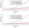Figure 1 Comparison of computational complexity (I): (a) number of multiplications; (b) number of additions. Four curves in (a) show the maximum and minimum multiplication requirements for the component-wise recursion method and the direct transformation method for a required Zernike component at one (x, y) position; the same applies to four curves in (b) for addition operations.

The above performance evaluation makes sense in theory, but calculating a single component is not so common in practice. In contrast, preparing all components from order 0 to order n is necessary for surface/wavefront reconstruction and analysis. The implementation of the corresponding methods significantly influences the final performance assessment. Two further aspects must be considered: 1) the reuse of lower-order results; 2) the use of modern computer hardware such as SIMD (Single-Instruction-Multiple-Data) technique and Cache-hierarchy. Block-wise recursion offers a direct route to modern, hardware-compatible implementations. Another computational performance comparison was performed between the component-wise recursive calculation method mentioned above and the block-wise recursive calculation method. Figure 2 shows the advantage of the latter method. Both methods were implemented and tested in the same MATLAB environment (DELL laptop, Intel(R) Core(TM) i5-1245U, 16GB RAM, 128MB Intel(R) UHD Graphics, Windows-11 OS, MATLAB-R2020b 64-bit) without any special coding optimization. Although this is only a preliminary assessment, the block-wise recursive method shows better computational performance, scaling linearly with the polynomial order while the component-wise recursive method appears to be exponentially relevant. This advantage stems from the inherent compatibility between the block-wise recursive method and modern hardware technology in civilian commercial computers.

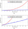Figure 2 Comparison of computational complexity (II): Time elapsed for generating all Zernike components up to order 99 using component-wise recursion (red) compared to block-wise recursion (blue): (a) the comparison; (b) further details on the elapsed time of block-wise recursion (with y-axis ≤1.5 ms). The comparison was performed for one (x, y) position, and the elapsed time is measured in millisecond (10−3 s).

4.2 Computational accuracy: a preliminary evaluation

In addition to the computational performance test described above, the computational accuracy was also compared using 120 spatial positions taken from 5 radius positions times 24 azimuth positions (see Fig. 3a). For each spatial position, all Zernike components from order 0 to order 99 were calculated using both the component-wise recursive method mentioned above ([7]) and the block-wise recursive method based on Pascal’s triangle (Eq. (12)). For each order, the maximum absolute difference between the results of both methods was recorded; thus, a difference curve along polynomial orders was created for each position. All 120 curves were recorded during the test. They are shown in Figure 3 in two versions: the raw difference curves (b) and their logarithmic (log10) version (c).

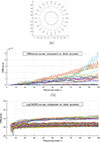Figure 3 Accuracy assessment of the block–wise recursion compared to the component-wise recursion (Andersen’s method [7]) for calculating Zernike basis functions: (a) 120 test positions from a circular region with five radii (1.00, 0.96, 0.88, 0.72, 0.40) and 24 uniformly distributed azimuth angles; (b) 120 difference curves (color–coded) with respect to the polynomial orders, each curve representing the maximum absolute differences between two sets of Zernike components along the orders from 0 to 99 for a position in (a); (c) the logarithmic representation (log10) of the corresponding curves in (b), of which 17 curves are distinguished from the others by their difference value of over 3 × 10−15 and whose corresponding positions all lie on the unit circle.

The comparison results show an absolute difference of less than 6 × 10⁻¹⁴, with the maximum absolute difference exceeding 3 × 10⁻¹⁵ at 17 positions on the unit circle from order 50 onwards. This preliminary result confirmed our expectation that the block-wise recursive method can be interpreted as equivalent to the component-wise recursive method, although the former is proposed on the basis of one Pascal triangle and the latter was developed from the TTRR relationship in orthogonal polynomials.

Naturally, the question arises as to the above 17 positions on the unit circle: which method is closer to the truth? Recursive methods (component-wise and block-wise recursion) were further compared with the direct transformation method (Eq. (10)). Unlike that the two recursive methods, which were fully implemented in MATLAB with double precision, the direct transformation method requires additional support from an external library for “arbitrary-precision-arithmetic” due to the rapidly increasing integer values (i.e., binomial factors) for polynomials of order higher than 50. The comparison results for the six positions with the largest deviations, all located on the unit circle, are shown in Figure 4. It is evident that for both recursive methods, all deviations are smaller than approximately 4 × 10⁻¹³ compared to the direct transformation method.

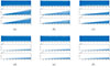Figure 4 Accuracy comparisons (a)–(f) at six positions on the unit circle: (x, y) ≈ (−0.5000000, −0.8660254), (−0.7071068, −0.7071068), (−0.5000000, 0.8660254), (0.5000000, 0.8660254). (0.5000000, −0.8660254), and (−0.8660254, −0.5000000). Each comparison includes three curves: the one above for 5050 Zernike components of orders 0 to 99, calculated using the direct transformation method, as the comparison reference; the middle one for the absolute difference of the component-wise recursive method to the reference; and the curve below for the block-wise recursive method. All difference curves are shown with the same value scale: ≤4 × 10−13.

It should be noted that this work does not constitute a definitive assessment of the accuracy of one method compared to others, but rather a preliminary evaluation to support the conceptual investigation of the relationship between Zernike polynomials and Pascal’s triangle. Further evaluations with more detailed application scenarios are to be expected, as the difference curves reveal some order-dependent structural information which, although very small, is not random noise.

4.3 Memory requirement

Memory requirements are often a critical factor in development due to detailed application scenarios. This work offers high flexibility for practical system/algorithm development: Block-wise recursive computation for generating basis functions requires no additional memory; similarly, virtually no additional memory is needed for surface/wavefront analysis, which uses transformation matrices for coefficient operations and derivative computations, since all transformation matrices can be rapidly computed by block-wise recursive algorithms, e.g., equation (11) for the forward coordinate system transformation in Zernike computations.

5 Conclusion

In this work, the computation of Zernike basis functions was divided into two parts: the part irrelevant to the coordinate values and the part relevant to the coordinate values. The first part comprises the computation of the coordinate transformation along with an orthogonalization process (based on homogeneous xy polynomials). This leads to two cases of block-wise recurrence in the coordinate-independent Zernike computation. The use of these two block-wise recurrences, supported by Pascal triangle, enables a block-wise direct transformation method and a block-wise recursive computation method for Zernike polynomials. The latter is more suitable for computing basis functions, while the former is better suited for operations and analyses of surfaces using their polynomial coefficients. Theoretically, this significantly improves computational speed, reduces memory requirements, and increases application flexibility without compromising accuracy. Optical applications can benefit from these new insights.

This work provides a solid starting point for further theoretical and application-specific studies, such as a comprehensive evaluation of computational complexity, a dedicated algorithmic accuracy/stability investigation, and application-oriented algorithm design, Zernike analysis with non-circular pupil, fast higher-order derivatives of a surface described by Zernike polynomials, etc. It is also valuable for discovering similar cases of block-wise recurrence in other orthogonal polynomials constructed using the Gram-Schmidt process.

Funding

This research received no external funding.

Conflicts of interest

The authors declare no conflicts of interest in regards to this article.

Data availability statement

The underlying data can be provided by the authors upon reasonable request.

References

Appendix A: Mathematical proofs

A.1 Pascal triangle supported block-wise recurrence in Zernike polynomials

The Zernike radial polynomial has its binomial form (Eq. (8)). Defining n = 2j, m = 2l for even orders and n = 2j + 1, m = 2l + 1 for odd orders, and defining two intermediate variables J _k  = j − k and J _2k  = 2J _k , we obtain$$\{\begin{array}{ll}{R}_{2j}^{2l}& =\sum _{k=0}^{j-l}\mathrm{}(-1{)}^k\left(\begin{array}{l}{J}_{2k}+k\\ J_{2k}\end{array}\right)\left(\begin{array}{l}{J}_{2k}\\ J_k+l\end{array}\right)({\rho }^2{)}^{J_k}\\ R_{2j+1}^{2l+1}& =\rho \sum _{k=0}^{j-l}\mathrm{}(-1{)}^k\left(\left(\begin{array}{l}{J}_{2k}+k\\ J_{2k}\end{array}\right)+\left(\begin{array}{l}{J}_{2k}+k\\ J_{2k}+1\end{array}\right)\right)\left(\left(\begin{array}{l}{J}_{2k}\\ J_k+l\end{array}\right)+\left(\begin{array}{l}{J}_{2k}\\ J_k+l+1\end{array}\right)\right)({\rho }^2{)}^{J_k}\end{array}.$$(A.1)

Further defining $w_k^e=\left(\begin{array}{l}{J}_{2k}+k\\ J_{2k}\end{array}\right)$, $w_k^o=w_k^e+\left(\begin{array}{l}{J}_{2k}+k\\ J_{2k}+1\end{array}\right)$, $t_{\mathrm{lk}}^e=\left(\begin{array}{l}{J}_{2k}\\ J_k+l\end{array}\right)$, and $t_{\mathrm{lk}}^o=t_{\mathrm{lk}}^e+\left(\begin{array}{l}{J}_{2k}\\ J_k+l+1\end{array}\right)$, we obtain$$\{\begin{array}{ll}{R}_{2j}^{2l}=& \sum _{k=0}^{j-l}\mathrm{}(-1{)}^k{w}_k^e{t}_{\mathrm{lk}}^e({\rho }^2{)}^{J_k}\\ R_{2j+1}^{2l+1}=\rho & \sum _{k=0}^{j-l}\mathrm{}(-1{)}^k{w}_k^o{t}_{\mathrm{lk}}^o({\rho }^2{)}^{J_k}\end{array}.$$(A.2)

In particular, we have $w_k^e=\left(\begin{array}{l}{J}_{2k}+k\\ J_{2k}\end{array}\right)=\left(\begin{array}{l}2j-k\\ k\end{array}\right)$, for which we obtain a vector by continuously increasing k by 1 from 0 to k = j − l, provided $w_{\left\{k\right\}}^e=\left[\begin{array}{llll}\left(\begin{array}{l}2j\\ 0\end{array}\right)& \left(\begin{array}{l}2j-1\\ 1\end{array}\right)& \cdots & \left(\begin{array}{l}j+l\\ j-l\end{array}\right)\end{array}\right]$ as a row vector, where 2j = n for even orders and l ≤ j; we also have $w_k^o=w_k^e+\left(\begin{array}{l}{J}_{2k}+k\\ J_{2k}+1\end{array}\right)=\left(\begin{array}{l}2j-k\\ k\end{array}\right)+\left(\begin{array}{l}2j-k\\ k-1\end{array}\right)=\left(\begin{array}{l}2j+1-k\\ k\end{array}\right)$, provided $w_{\left\{k\right\}}^o=\left[\begin{array}{llll}\left(\begin{array}{l}2j+1\\ 0\end{array}\right)& \left(\begin{array}{l}2j\\ 1\end{array}\right)& \cdots & \left(\begin{array}{l}j+1+l\\ j-l\end{array}\right)\end{array}\right]$, where 2j + 1 = n for odd orders and l ≤ j. Either $w_{\left\{k\right\}}^e$ or $w_{\left\{k\right\}}^o$ denotes a corresponding anti-diagonal vector in a left-aligned n-row Pascal triangle (e.g., Table 2 for n ≤ 6). For one even (or odd) order, $w_{\left\{k\right\}}^e$ (or $w_{\left\{k\right\}}^o$) depends on a single variable k and is independent of l or m.

Meanwhile, for an even order n = 2j, we have $t_{\mathrm{lk}}^e=\left(\begin{array}{l}{J}_{2k}\\ J_k+l\end{array}\right)=\left(\begin{array}{l}2(j-k)\\ (j-k)+l\end{array}\right)$, where $t_{\mathrm{lk}}^e{|}_{k=0}=\left(\begin{array}{l}2j\\ j+l\end{array}\right)$ subject to k = 0; continuously increasing k by 1 till k = j − l, we obtain a row vector $t_{l\left\{k\right\}}^e=\left[\begin{array}{lllll}\left(\begin{array}{l}2j\\ j+l\end{array}\right)& \left(\begin{array}{l}2j-2\\ j-1+l\end{array}\right)& \left(\begin{array}{l}2j-4\\ j-2+l\end{array}\right)& \cdots & \left(\begin{array}{l}2l\\ 2l\end{array}\right)\end{array}\right]$ with respect to a particular l, and obtain an anti-upper-triangular matrix for all the 0 ≤ l ≤ j, as$$T_{n=2j}\left(t_{\mathrm{lk}}^e\right)=t_{\left\{l\right\}\left\{k\right\}}^e={\left[\begin{array}{llllll}\left(\begin{array}{l}2j\\ j\end{array}\right)& \left(\begin{array}{l}2j-2\\ j-1\end{array}\right)& \left(\begin{array}{l}2j-4\\ j-2\end{array}\right)& \cdots & \left(\begin{array}{l}2\\ 1\end{array}\right)& \left(\begin{array}{l}0\\ 0\end{array}\right)\\ \left(\begin{array}{l}2j\\ j+1\end{array}\right)& \left(\begin{array}{l}2j-2\\ j\end{array}\right)& \left(\begin{array}{l}2j-4\\ j-1\end{array}\right)& \cdots & \left(\begin{array}{l}2\\ 2\end{array}\right)& \\ \left(\begin{array}{l}2j\\ j+2\end{array}\right)& \left(\begin{array}{l}2j-2\\ j+1\end{array}\right)& \left(\begin{array}{l}2j-4\\ j\end{array}\right)& \cdots & & \\ \cdots & \cdots & \ddots & & & \\ \left(\begin{array}{l}2j\\ 2j-2\end{array}\right)& \left(\begin{array}{l}2j-2\\ 2j-2\end{array}\right)& & & & \\ \left(\begin{array}{l}2j\\ 2j\end{array}\right)& & & & & \end{array}\right]}_{(j+1)\times (j+1)}.$$(A.3)

References

- Lakshminarayanan V, Fleck A, Zernike polynomials: a guide, J. Modern Opt. 58(7), 545–561 (2011). https://doi.org/10.1080/09500340.2011.633763. [Google Scholar]
- Schwiegerling J, Description of Zernike Polynomials, 2016. https://wp.optics.arizona.edu/visualopticslab/wp-content/uploads/sites/52/2016/08/Zernike-Notes-15Jan2016.pdf. [Google Scholar]
- Niu K, Tian C, Zernike polynomials and their applications, J. Opt. 24(12), 1–54 (2022). https://doi.org/10.1088/2040-8986/ac9e08. [Google Scholar]
- Born M, Wolf E, Bhatia AB, Principles of optics: Electromagnetic theory of propagation, interference and diffraction of light, 7th ed., Vol. 523 (Cambridge University Press, Cambridge, UK, 1999). ISBN 978-0-521-64222-4. https://books.google.de/books?id=nUHGpfNsGyUCq=Zernikeredir_esc=y#v=snippetq=Zernikef=false. [Google Scholar]
- Zernike F, Beugungstheorie des schneidenver-fahrens und seiner verbesserten form, der phasenkontrastmethode, Physica 1(7–12), 689–704 (1934), https://doi.org/10.1016/S0031-8914(34)80259-5. [Google Scholar]
- Shakibaei BH, Paramesran R, Recursive formula to compute Zernike radial polynomials, Opt. Lett. 38(14), 2487–2489 (2013). https://doi.org/10.1364/OL.38.002487. [Google Scholar]
- Andersen TB, Efficient and robust recurrence relations for the Zernike circle polynomials and their derivatives in Cartesian coordinates, Opt. Exp. 26(15), 18878–18896 (2018). https://doi.org/10.1364/OE.26.018878. [Google Scholar]
- van Brug H.H. (1997) Efficient Cartesian representation of Zernike polynomials in computer memory, Proc. SPIE: Fifth Int. Topical Meet. Educ. Train. Opt. 382–392, https://doi.org/10.1117/12.294412. [Google Scholar]
- Mathar RJ, Zernike basis to Cartesian Transformations, Serbian Astron. J. 179, 107–120 (2009). https://doi.org/10.2298/SAJ0979107M. [Google Scholar]
To our knowledge, block-wise recurrence in Zernike calculations has hardly been addressed in the literature, although there is a long history of intensive studies on Zernike polynomials.
The mathematical derivation in this section briefly proves the two previously mentioned cases of block–wise recurrence in Zernike computations without order restriction. Further details can be found in Appendix A.
This arrangement corresponds to the OSA/ANSI standard indices for Zernike polynomials [3].
Table B1 in Appendix B gives 𝓣, Table B2 its inverse 𝓣−1, each up to order 6.