© The Author(s), published by EDP Sciences, 2025

1 Introduction

Along with the developments of the semiconductor industry, the minimum circuit width has been expected to be a few nanometers [1]. These trends lead to the shape error of mirrors in semiconductor manufacturing machine (EUV lithography machine) must be within 50 pm [2]. For such high-resolution measurement, the laser interferometry has been a good candidate because the measurement result has traceability to the definition of SI unit “meter”.

The resolution of the displacement measuring interferometer has reached a few tens of picometer. Here, some examples (“Heterodyne”, “Homodyne” and “Sinusoidal phase modulation (SPM)” interferometers) which measure physical mirror displacements in laboratory environment are shown.

1. Heterodyne interferometer: Hsu et al. reported a demodulation (phase-meter) algorithm using a digital phase-locked loop (PLL) implemented in field programmable gate array (FPGA) [3]. Yokoyama et al. reported spatially separated interferometer to reduce polarization mixing effect included in the interference signal [4]. Nguyen et al. reported a digital phase-locked loop implemented in FPGA for improving sensitivity of the phase-meter [5, 6]. Kokuyama et al. reported introducing an oversampling for noise reduction using FPGA [7].

2. Homodyne interferometer: Pisani et al. reported a multi-folded configuration for increasing the basic resolution [8, 9]. Hori et al. reported a high sensitivity optic configuration and a correction of Lissajous diagram [10].

3. SPM interferometer [11, 12]: Higuchi et al. reported a high-speed modulation and a filtering for band limiting [13]. Through the development of high precision heterodyne interferometry [5, 6] and SPM interferometry [13] by our group, it was found that air fluctuations in the interferometer optical path are serious problems. The fluctuations were considered as temporal and spatial variations of the refractive index, which caused dynamic wavefront aberration leading dynamic 2-dimensional (2-D) in-plane displacement. Precise observation of air fluctuation in such situation has been strongly necessary to improve the resolution of the displacement measurement in air.

Shack-Hartmann sensor is popular to measure wavefront aberration of optical paths [14]. It measures the wavefront by focusing the incident beam on a camera using a micro lens array. The resolution and measurable range depend on the pixel size and effective focal length of the lens, and the measurement speed depends on the camera frame rate. Some Shack-Hartmann sensors can measure at around 1 kfps or a resolution of λ/200 in real-time [15]. However, Shack-Hartmann sensors are not capable of measuring the wavefront (i.e., 2-D in-plane displacement) of every single camera pixel. Surface profile interferometers such as Fizeau interferometers are considered capable of measuring the wavefront (=2-D in-plane displacement) at each pixel of the camera at a hundred nano meter range [16, 17]. Although the surface profile measurement resolution with Fizeau interferometers has reached sub-nm, the sampling rate is slow, at most several 10 Hz. For the air fluctuation measurement with Shack-Hartmann sensors or Fizeau interferometers, both the measurement resolution and the measurement speed are not enough. The authors believe that a 2-D in-plane displacement measurement system with a sampling rate of several kHz or higher and a resolution of sub-nm or less displacement per camera pixel is needed to study air fluctuations for precision interferometry and astronomical observations.

In this paper, to solve the above problem, we propose a SPM interferometer for 2-D in-plane displacement measurement with sub-nm resolution and fast speed sampling rate of 5 kHz. The interferometer consists of a Michelson type interferometer incorporating an electric-optic modulator (EOM) with a modulation frequency of 5 kHz and a high-speed camera (HSC) synchronized to a clock signal at a frequency of 60 kHz, 12 times the modulation frequency. Phase demodulation of all pixels in the camera is performed by acquiring the interference signal to that pixel synchronously with the sampling signal and performing a specific addition and subtraction between the signals obtained synchronously. By applying this procedure to all pixels in the camera, 2-D in-plane displacements can be obtained. In this paper, we report on the measurement equipment, the demodulation principle, the pre-filter for noise reduction and experimental results.

2 Principle

The schematic diagram of the SPM interferometer with an external EOM configuration is shown in Figure 1. A light source outputs a single frequency and a linear polarized beam. The polarization angle is controlled to 45° against to p-polarization axis (along with x-axis) using a half wave plate (HWP) and a polarizer (P). The beam passes through an EOM which modulates phases of the beam in a sinusoidal way. It is noticed that the EOM modulates phases in both p-polarizing beam and s-polarizing beam with different modulation efficiencies. If p- and s-polarizations are 100% and is 31%, respectively, because the electro-optic coefficients of r₁₃ and r₃₃ are 9.6 fm/V and 30.9 fm/V in a LiNbO3 crystal used in the paper, respectively [18]. The difference results in phase modulation of 69%, thus this configuration has a lower phase modulation index than conventionally used configuration in which the EOM is inserted reference arm [19, 20].

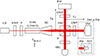Figure 1 Schematic diagram of SPM interferometer, HWP: Half wave plate, P: Polarizer, EOM: Electro-optic modulator, BE: Beam expander, PBS: Polarization beam splitter, QWP: Quarter wave plate, BS: Beam splitter, DM: Deformable mirror, HSC: High-speed camera, PM: Plane mirror with piezoelectric transducer (PZT). DM and PM are exclusively utilized.

The beam diameter is around 2 mm at the EOM aperture. To measure a mirror deformation with the area around ten-millimeter diameter, the 10 times beam expander (BE) is inserted. We use unbalanced arm length Michelson interferometer with polarizing optics. The beam from the BE is split into a reference optical path L_R and a target optical path L_T by the PBS. A reference mirror (RM) is mechanically fixed to base frame. A deformable mirror (DM) or a plane mirror (PM) with piezoelectric transducer (PZT) is employed as a target mirror. Beams which are split by the polarizing beam splitter (PBS) are reflected from these mirrors, then go to HSC and interfere with each other. The phase modulation and the mirror deformation with DM (or 2-D in-plane displacement with PM) generate a periodic interference fringe change like a beat fringe in heterodyne interferometer. We represent the spatial phase difference ϕ(x, y, t) to be measured as equation (1),$$\varphi \left(x, y, t\right)=\frac{4\pi n}{\lambda }\left\{L_{\mathrm{R}}\left(x, y, t\right)-L_{\mathrm{T}}\left(x, y, t\right)\right\}=\frac{4\pi }{\lambda }n\left(x, y, t\right)\Delta L\left(x, y, t\right),$$(1)where x, y, t, λ, n(x, y, t) ∆L(x, y, t) are pixel positions along x- and y axes at sensor of camera, time, vacuum wavelength, air refractive index and 2-D in-plane displacement to be measured which corresponds to the path difference out of flat plane, respectively. It is noted that the lateral resolution corresponded to the pixel pitch of the camera is 20 μm in following experiments. The interference fringe I_HSC(x, y, t) at HSC is represented by equation (2).$$I_{\mathrm{HSC}}\left(x, y, t\right)={E_{\mathrm{T}}}^2+{E_{\mathrm{R}}}^2+2E_{\mathrm{T}}{E}_{\mathrm{R}}\cos \left\{\varphi \left(x, y, t\right)+m\sin {\omega }_{m}t\right\},$$(2)where E_T, E_R, ω_m and m are complex amplitudes in target and reference paths, a modulation angular frequency and a modulation index. The modulation index m is represented as (see Appendix),$$m=\frac{\pi L_{\mathrm{EOM}}}{\lambda d_{\mathrm{EOM}}}\left({n_1}^3{\gamma }_{13}-{n_3}^3{\gamma }_{33}\right)V_{\mathrm{E}\mathrm{OM}}{K}_{\mathrm{EOM}}\left(∆t\right),$$(3)where L_EOM, d_EOM, V_EOM, K_EOM and ∆t = |L_R − L_T|/c, c are a length and a thickness of the EOM crystal, an applied voltage to the EOM, a modified term due to optical path difference, delay time and speed of light in vacuum, respectively. The modified term K_EOM(∆t) ≅ 1, when the optical path difference is within 1 m in case of the modulation frequency is 5 kHz (see Appendix). The modulation index m can be fixed by determining V_EOM.

The interference signal can be rewritten using Bessel function as$$\begin{array}{c}{I}_{\mathrm{HSC}}\left(x, y, t\right)={E_{\mathrm{T}}}^2+{E_{\mathrm{R}}}^2+2E_{\mathrm{T}}{E}_{\mathrm{R}}\cos \varphi \left(x, y, t\right)\left\{J_0\left(m\right)+2{\sum }_{k=1}^{\infty }{J}_{2k}\left(m\right)\cos \left(2k{\omega }_{m}t\right)\right\}\\ -2E_{\mathrm{T}}{E}_{\mathrm{R}}\sin \varphi \left(x, y, t\right)2{\sum }_{k=1}^{\infty }{J}_{2k-1}\left(m\right)\sin \left\{\left(2k-1\right){\omega }_{\mathrm{m}}t\right\},\end{array}$$(4)where J_k(m) is the Bessel function of order k with modulation index m. It is revealed that the interference signal is a sum of harmonic waves. It should be noted that the amplitude of even-order harmonics includes cos ϕ(x, y, t), while the amplitude of odd-order harmonics includes sin ϕ(x, y, t). The phase ϕ(x, y, t) can be obtained using amplitudes of even and odd order harmonics.

To extract the sin ϕ(x, y, t) and cos ϕ(x, y, t) terms from the interference signal, a demodulation (phase-meter) algorithm is implemented in a personal computer (PC) connected to HSC. The division of the interference signal into harmonics from the 0th to 6th order at a given sampling rate is shown in Figure 2. (Note, in Fig. 2, that the amplitude of the harmonics is not proportional to the magnitude of the Bessel function.) In the demodulation algorithm, the interference signal is sampled at 12 equal intervals (12 sampling points) in 1 modulation period (2π/ω_m) synchronizing to the modulation frequency (as shown by black dots). The 0th sampling point is the zero-crossing point at which the first harmonic changes from negative to positive. The values at sampling points 0, 3T_m/12, 6T_m/12 and 9T_m/12 for 2nd harmonic correspond to peaks or valleys. Similarly, values at sampling points T_m/12, 3T_m/12, 5T_m/12, 7T_m/12, 9T_m/12 and 11T_m/12 for 3rd harmonic correspond to peaks or valleys. Therefore, cos ϕ(x, y, t) and sin ϕ(x, y, t) in equation (4) can be calculated by adding and subtracting the peak and valley values of the second and third harmonics, respectively, using the following equations.$$16A J_2\left(m\right)\cos \left(\frac{4\pi n∆L}{\lambda }\right)=I\left(0\right)-I\left(\frac{3}{12}{T}_m\right)+I\left(\frac{6}{12}{T}_m\right)-I\left(\frac{9}{12}{T}_m\right)\equiv I_{\cos },$$(5) $$-24A{J}_3\left(m\right)\sin \left(\frac{4\pi n∆L}{\lambda }\right)=I\left(\frac{1}{12}{T}_m\right)-I\left(\frac{3}{12}{T}_m\right)+I\left(\frac{5}{12}{T}_m\right)-I\left(\frac{7}{12}{T}_m\right)+I\left(\frac{9}{12}{T}_m\right)-I\left(\frac{11}{12}{T}_m\right)\equiv I_{\sin }.$$(6)

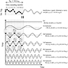Figure 2 Sampling timing in phase demodulation algorithm.

In equations (5) and (6), only 2nd and 3rd harmonics (Bessel functions) are considered. If the modulation index m is larger than 3 rad, higher harmonics (higher Bessel functions) may be included in cos ϕ(x, y, t) and sin ϕ(x, y, t) terms. Table 1 shows which harmonics are mixed in the calculations of equations (5) and (6) at the modulation index m = 3.14 rad. In the table, from the left column, the harmonic order k, the target harmonic (sine or cosine), J_k(m)/J₂(m) (ratio of kth-order Bessel function to 2nd-order Bessel function), J_k(m)/J₃(m) (ratio of kth-order Bessel function to 3rd-order Bessel function), the harmonic mixed in equation (5) (I_cos) (1: in-phase, 0: not mixed), and harmonics mixed in equation (6) (I_sin) (0: not mixed, −1: in-phase). Table 1 shows that harmonics of the 0th, 1st, 4th, 5th, 7th, and 8th orders have no effect on the calculations of equations (5) and (6) for cos ϕ(x, y, t) and sin ϕ(x, y, t). In the cos ϕ(x, y, t), the 2nd, 6th, and 10th harmonics are mixed in phase, and the ratio of the 6th and 2nd magnitudes is J₆(m)/J₂(m) ≈ 2.988%, which is not negligible. 10th harmonics are negligible with a similar ratio of J₁₀(m)/J₂(m) ≈ 0.004%. In the calculation of sin ϕ(x, y, t) in equation (6), the 9th harmonic is introduced in the opposite phase, but the same ratio of J₉(m)/J₃(m) ≈ 0.037% is negligible. Based on the above discussion, rewriting equation (5) for a modulation index of m = 3.14 rad, we obtain$$I_{\cos }=I\left(0\right)-I\left(\frac{3}{12}{T}_m\right)+I\left(\frac{6}{12}{T}_m\right)-I\left(\frac{9}{12}{T}_m\right)=16A \left\{J_2\left(m\right)+J_6\left(m\right)\right\}\cos \left(\frac{4\pi n∆L}{\lambda }\right).$$(7)

When the modulation index m = 3.14 rad, we can obtain 16{J₂(m) + J₆(m)}=24J₃(m), so that |I_cos| = |I_sin|. Then we can illustrate a Lissajous diagram of a perfect circle using I_cos and I_sin as lateral and vertical axes. The phase $\varphi \left(x, y, t\right)=\frac{4\pi n∆L}{\lambda }$ can be calculated by arctangent of I_cos and I_sin. In the case of 2-D in-plane displacement measurement, interference signals are recorded for all pixels of HSC. However, due to the huge amount of image data, it is currently impossible to calculate and output the displacement of each pixel in real time. Most current HSCs store the captured video data in the camera’s internal memory and transfer the video data to a PC or FPGA when the image capture is completed. A linear image sensor can transfer the output signals of each pixel to an analog-to-digital converter incorporated in a PC or an FPGA in real time [21], and phase (displacement) measurement with the linear image sensor is considered possible in real time. Similarly, if the output signal of each pixel of a HSC can be transferred in real time to an FPGA capable of large-scale, high-speed computation via a high-speed line such as an optical fiber [22], real-time measurement may be possible with the HSC. The calculations of the 2-D in-plane displacement of all pixels of the HSC used in the experiments are performed in post-processing.

However, it is possible to apply a pre-filter to the interference signal before calculations of equations (6) and (7), albeit in post-processing. To improve the resolution, we introduce the feedback type comb filter for pre-filtering the interference signal. Since the output of a SPM interferometer contains only the harmonics of the modulation signal, a comb filter that transmits only its harmonic components is employed as a prefilter. The block diagram of the comb filter is shown in Figure 3. Its Bode diagram with D = 12, K_i = 0.9 and the cut-off frequency = 145 Hz is shown in Figure 4. The feedback type comb filter has sharp pass bands at 5 kHz, 10 kHz, 15 kHz, …. Due to matching the pass bands and harmonics, we can decrease the noise included in the interference signal.

Figure 3 Block diagram of the comb filter.

Figure 4 Bode diagram of the comb filter, (a) the amplitude response, (b) the phase response.

3 Experiment

The experimental setup is illustrated in Figure 5. A He-Ne laser (Spectra-Physics, 117A) is used as a light source. With the limitation of optical bread board size, some mirrors are used to steer the beam into the homemade EOM (d = 3 mm, W = 3 mm, l = 70 mm) and the interferometer. The reference arm length is designed minimum due to the external EOM configuration. The interferometer flame is made of low expansion steel (Nippon Chuzo, LEX-ZERO) to eliminate the effect of temperature fluctuation. A DM (Thorlabs, DMP40/M) which is a multi-segmented piezo driven deformable mirror, is utilized in 2D in-plane displacement. Although the DM has 40 segments, an area of 8 segments located in the center of the DM is targeted due to the beam diameter. PM movements generated by PZT driven linear stage are also measured in performance inspection and 2-D in-plane displacement. DM and PM were exclusively utilized in experiments. The interferometer, DM, PM with linear stage and HSC (Photron, FASTCAM Mini AX200 AOFT1) are located on the breadboard which is also made of low expansion steel. The breadboard is placed on the anti-vibration table. Conditions on experiments are shown in Table 2. To design the bandwidth higher than WFS, the modulation frequency is selected to 5 kHz, leading to the frame rate of 60 kHz and pixel area of (128, 128) or (256, 256) (equal to area of 2.56 mm × 2.56 mm or 5.12 mm × 5.12 mm).

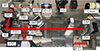Figure 5 Experimental setup.

4 Results

In this section, some measurement results are discussed. We conduct 2-D in-plane displacement measurements using plane mirror movement and mirror deformation as demonstrative measurements. Triangular waveform movement of PM with the amplitude of 400 nm and frequency of 5 Hz is shown Figure 6. Lissajous diagram using I_cos and I_sin at (60, 60) pixel in HSC is shown in Figure 6a. In Figure 6a, a circular Lissajous diagram is obtained by adjusting the voltage V_EOM using equation (3), it means that the estimation of the modulation index m shown in equation (3) and Appendix is valid. The demodulated single point displacement from Lissajous diagram at (60, 60) pixel is shown in Figure 6b. The 2-D in-plane results are shown in Figure 6c. Figure 6 shows that the 2D in-plane displacement of the entire PM surface can be measured. Periodic interpolation uncertainties are observed in the demodulated displacements in Figure 6b. Determining the cause of this is the future challenge.

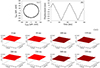Figure 6 Triangular displacement with 400 nm and 5 Hz, (a) Lissajous diagram at (60, 60) pixel, (b) demodulated displacement at (60, 60) pixel, (c) 2-D in-plane demodulated displacement.

We examine whether partial deformation of DM surface can be measured. As shown in Figure 7a, the DM surface is divided into 8 circumferential sections, with each section protruding 125 nm and its protrusion varying in a roulette-like fashion. Figure 7b shows the deformation of the DM surface. In Figure 7b, the yellow area in the figure shows that the protruding part (120 nm displacement) rotates with time. From Figure 7b, it can be seen that the time-varying surface deformation can be measured by the proposed method.

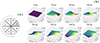Figure 7 DM displacement like roulette motion, (a) Segment structure of DM and its roulette motion, (b) 2-D in-plane result.

In the resolution inspection measurements, small movement of PM and noise floor are measured. To verify the effectiveness of the pre-filter, a comparison was made between using it and not using it. The filter condition is described in the above section. The result of mirror movement which is a square waveform with the amplitude of 2 nm and the frequency of 10 Hz are shown in Figure 8. The results without and with pre-filter are shown in Figures 8a and 8b, respectively. Without pre-filter, the noise amplitude is approximately as same as the displacement step. With pre-filter, the noise width is reduced to less than 0.5 nm. The intensity resolution of the HSC is 12 bits, so if the wavelength λ is 633 nm, the displacement resolution is λ/2(2¹² − 1) ≈ 77 pm. However, the resolution measured in Figure 8 is considerably worse than this. Resolution improvement is a future challenge.

Figure 8 2 nm displacement at (60, 60) pixel with comb filter, (a) without filter, (b) with filter.

The interferometer noise floor was measured with the PM stationary. The noise floor with frequency range from 0.5 Hz to 2.5 kHz is shown in Figure 9. In the figure, the black and gray lines show the noise floor results without and with the pre-filter, respectively. In the frequency range from 100 Hz to 2.5 kHz, the noise shape without pre-filter is flat at around $0.1 \mathrm{nm}/\sqrt{\mathrm{Hz}}$, while the noise shape with pre-filter decreases with increasing frequency. In the low frequency range from 0.1 Hz to 1 Hz, the noise increases with decreasing frequency. Reducing the noise floor to the theoretical resolution of the HSC is also the future challenge.

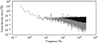Figure 9 Noise floor at (60, 60) pixel. Black line was without the pre-filter and gray line was with the pre-filter.

We measure air fluctuation in measurement path in case of the fixed plane mirror. A fan is used to generate a wind speed of approximately 1 m/s in a direction perpendicular to the optical axis. The measured 2-D in-plane result is shown in Figure 10a. A single point at (60, 60) pixel is shown in Figure 10b. The variation of the air turbulence causes tens of nanometer fluctuation. It is known that the air flow configuration to optical path caused fluctuation in displacement measurement, but the relationship between the beam wave front and the displacement had not been revealed. In Figure 10a, from 50 ms~350 ms, the high displacement locations (shown in yellow) appear to move randomly with time. Figure 10b shows that the time variation of the displacement of the central pixel fluctuates approximately 30 nm during 400 ms. Figures 10a and 10b show that the wavefront varies dynamically in time and space, resulting in the observed displacements. The next issue is the extent to which air fluctuations in turbulence can be measured using the proposed method.

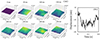Figure 10 Air flow turbulence of 1 m/s, (a) 2-D in-plane result, (b) at (60, 60) pixel.

5 Conclusion

In this paper, we introduced a SPM interferometer for nanometer order 2-D in-plane displacement measurement. HSC and PC based phase-meter were utilized for 2-D measurement. The configuration of the interferometer and the algorithm of the phase-meter (demodulation) were described. In experiment, displacement measurement with PM was conducted to inspect the noise characteristic and the resolution. PM movement and deformation of DM were measured. Noise reduction using pre-filter was also described and the sub-nanometer resolution was suggested. Since this interferometer was specifically designed for high-speed cameras, relatively huge optical components such as EOM, BE, and DM were introduced, resulting in a much longer optical path length than previously reported [13]. This may cause air fluctuations and noise due to the low stiffness of the mechanical components in the frequency range below 100 Hz. Shortening the optical path length of the interferometer and increasing the rigidity of the mechanical components may reduce these noise levels.

As future work, one improvement and one development may be attempted. The improvement is to modify the current interferometer configuration (optics and its arrangements) to improve mechanical stiffness, air fluctuation robustness, and interferometric resolution. The development is to increase the modulation frequency to 2 MHz using a high modulation frequency EOM and a high frame rate HSC.

Funding

We express our gratitude to the Research Fund of Japan Society for the Promotion of Science (Grant Number: 20H02042) for supporting this research. We would also like to thank Chuo Precision Industrial Co. Ltd., for valuable discussions.

Conflicts of interest

The authors declare that they have no conflict of interests.

Data availability statement

The research data associated with this article are included within the article.

Author contribution statement

Higuchi proposed the idea and the calculation, carried out the experiments, and wrote the manuscript. All co-authors participated in the discussion of the theory and experimental results. All authors read and approved of the final.

Glossary

2D Two dimensional, BE Beam expander, BS Beam splitter, DM Deformable mirror, EOM Electro-optic modulator, EUV Extreme ultraviolet, FPGA field programmable gate array, HSC High-speed camera, HWP Half wave plate, P Polarizer, PBS Polarization beam splitter, PLL Phase-locked loop, PM Plane mirror, PZT Piezoelectric transducer, QWP Quarter wave plate, SPM Sinusoidal phase modulation.

References

Appendix

The approximation in modulation index m calculation is explained in this section. The SPM interferometer described below uses EOM for phase modulation. The phase of the outgoing light from the EOM varies depending on the crystal orientation of the EOM, the direction of the applied voltage, and the polarization of the incident light. Figure A1 shows the considered arrangement. The E_EOM is the electrical field applied to EOM along with y axis (thickness direction). Due to the polarizer with 45-degree inclination, the electrical field of the incident beam to the EOM is written as$${\mathit{E}}_{\mathbf{1}}\left(z, t\right)=\left(\begin{array}{c}{E}_x\\ E_y\end{array}\right)=\left(\begin{array}{c}1\\ 1\end{array}\right)e^{i\left(\mathrm{kz}-\omega t+{\varphi }_0\right)}$$A1where, E_x, E_y t, k, ω, and ϕ₀ are electric fields along x and y axes time, wave number, angular frequency of the beam, and initial phase, respectively. EOM shifts the phase with refractive index of EOM, which efficiency are different in the axis direction. Amounts of the phase shift with applying voltage V are written as$${\varphi }_x=\frac{2\pi l}{\lambda }\left(n_1-\frac{{n_1}^3}{2}{\gamma }_{13}\frac{V_{\mathrm{EOM}}}{d} \right),$$A2 $${\varphi }_y=\frac{2\pi l}{\lambda }\left(n_3-\frac{{n_3}^3}{2}{\gamma }_{33}\frac{V_{\mathrm{EOM}}}{d}\right),$$A3where, l, λ, n₁, n₃, γ₁₃, γ₃₃, and V_EOM are the length of the EOM crystal, the wavelength, the refractive index of the EOM, the electro-optic coefficient of the EOM crystal and applied voltage to EOM, respectively. The refractive index n₁ and n₃ are not same in LiNbO3.The electrical field of the transmitted beam is written as$${\mathit{E}}_{\mathbf{2}}\left(z, t\right)=\frac{1}{\sqrt{2}}\left(\begin{array}{c}{e}^{i{\varphi }_x}\\ e^{i{\varphi }_y}\end{array}\right)e^{i\left(\mathrm{kz}-\omega t+{\varphi }_0\right)}.$$A4

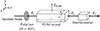Figure A1 Geometrical relationship between incident beam and EOM crystal.

If the y axis polarization beam goes to the reference arm and the x axis polarization beam goes to the target arm, the combined electrical field at HSC is written as$${\mathit{E}}_{\mathbf{3}}\left(z, t\right)=\frac{1}{\sqrt{8}}\left(\begin{array}{c}{e}^{i\left(2k{L}_{\mathrm{R}}+{\varphi }_x\right)}+e^{i\left(2k{L}_{\mathrm{T}}+{\varphi }_y\right)}\\ 0\end{array}\right)e^{i\left(-\omega t+{\varphi }_0\right)}.$$A5

The interference signal I could be written as$$I={\left|{\mathit{E}}_{\mathbf{3}}\left(z, t\right)\right|}^2=\frac{1}{4}+\frac{1}{4}\cos \left\{2k\left(L_{\mathrm{R}}-L_{\mathrm{T}}\right)+\left({\varphi }_x-{\varphi }_y\right)\right\}.$$A6

In case of L_R < L_T, the beam along with the x axis polarization delays $∆t=\frac{2n\left(L_{\mathrm{T}}-L_{\mathrm{R}}\right)}{c}$ compared to the beam along with the y axis polarization. The phase difference ϕ_x − ϕ_y by applying sinusoidal voltage V_EOM sin ω_mt is rewritten as$$\begin{array}{c}{\phi }_y\left(t\right)-{\phi }_x\left(t+∆t\right)=\frac{2\pi l}{\lambda }\left\{\left(n_1-\frac{{n_1}^3}{2}{\gamma }_{13}\frac{V_{\mathrm{EOM}}\sin {\omega }_{m}t}{d}\right)-\left(n_3-\frac{{n_3}^3}{2}{\gamma }_{33}\frac{V_{\mathrm{EOM}}\sin {\omega }_m\left(t+∆t\right)}{d}\right)\right\}\\ =\frac{2\pi l}{\lambda }\left\{\left(n_1-n_3\right)+\frac{V_{\mathrm{EOM}}}{2d}\left({n_1}^3{\gamma }_{13}\sin {\omega }_{m}t-{n_3}^3{\gamma }_{33}\sin {\omega }_m\left(t+∆t\right)\right)\right\}.\end{array}$$

Using the relationship of $a\sin \theta -b\sin \left(\theta +∆\right)=\sqrt{{\left(a-b\cos ∆\right)}^2+{\left(b\sin ∆\right)}^2}\sin \left\{\theta +\mathrm{atan}\frac{-b\sin ∆}{a-b\cos ∆}\right\}$, the phase difference is rewritten as$${\phi }_y\left(t\right)-{\phi }_x\left(t+∆t\right)=\frac{2\pi l}{\lambda }\left(n_1-n_3\right)+m\sin \left\{{\omega }_{m}t+\theta \right\},$$A7where,$$m=\frac{\pi }{\lambda }\frac{V_{\mathrm{EOM}}}{d}\sqrt{{\left({n_1}^3{\gamma }_{13}-{n_3}^3{\gamma }_{33}\cos {\omega }_m∆t\right)}^2+{\left({n_3}^3{\gamma }_{33}\sin {\omega }_m∆t\right)}^2},$$A8 $$\theta =\mathrm{atan}\frac{-{n_3}^3{\gamma }_{33}\sin {\omega }_m∆t}{{n_1}^3{\gamma }_{13}-{n_3}^3{\gamma }_{33}\cos {\omega }_m∆t}.$$A9

Applying the experimental condition of f_m = 5 kHz and L_R – L_T = 350 mm, ω_m ∆t ≈ 7.3 × 10 ⁻⁵, and the modulation index m is rewritten as$$m=\frac{\pi l}{\lambda d}\sqrt{{\left({n_1}^3{\gamma }_{13}-{n_3}^3{\gamma }_{33}\right)}^2+{\left({n_3}^3{\gamma }_{33}{\omega }_m∆t\right)}^2} V_{\mathrm{EOM}},$$A10

The term (n₁³ γ₁₃ − n₃³ γ₃₃)² is stational. The term n₃³ γ₃₃ω_m∆t must be considered to designe appropriate phase modulation. We rewrite the modulation index as equation (3) using K_EOM(∆t) for simple representation. K_EOM(∆t) is written as$$K_{\mathrm{EOM}}\left(∆t\right)=\sqrt{1+\frac{{\left({n_3}^3{\gamma }_{33}{\omega }_m∆t\right)}^2}{{\left({n_1}^3{\gamma }_{13}-{n_3}^3{\gamma }_{33}\right)}^2}}.$$A11

The relationship between the optical path difference and K_EOM(∆t) at the modulation frequency f_m(= ω_m/2π) of 5 kHz is shown in Figure A2. The value of {1 − K_EOM(∆t)} at 350 mm is less than 10⁻⁴ order then the effect of delay time ∆t is ignored.

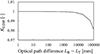Figure A2 Relationship between LR − LT and KEOM(∆t) if the modulation frequency fm is 5 kHz.

All Tables

All Figures

	Figure 1 Schematic diagram of SPM interferometer, HWP: Half wave plate, P: Polarizer, EOM: Electro-optic modulator, BE: Beam expander, PBS: Polarization beam splitter, QWP: Quarter wave plate, BS: Beam splitter, DM: Deformable mirror, HSC: High-speed camera, PM: Plane mirror with piezoelectric transducer (PZT). DM and PM are exclusively utilized.
In the text

	Figure 2 Sampling timing in phase demodulation algorithm.
In the text

	Figure 3 Block diagram of the comb filter.
In the text

	Figure 4 Bode diagram of the comb filter, (a) the amplitude response, (b) the phase response.
In the text

	Figure 5 Experimental setup.
In the text

	Figure 6 Triangular displacement with 400 nm and 5 Hz, (a) Lissajous diagram at (60, 60) pixel, (b) demodulated displacement at (60, 60) pixel, (c) 2-D in-plane demodulated displacement.
In the text

	Figure 7 DM displacement like roulette motion, (a) Segment structure of DM and its roulette motion, (b) 2-D in-plane result.
In the text

	Figure 8 2 nm displacement at (60, 60) pixel with comb filter, (a) without filter, (b) with filter.
In the text

	Figure 9 Noise floor at (60, 60) pixel. Black line was without the pre-filter and gray line was with the pre-filter.
In the text

	Figure 10 Air flow turbulence of 1 m/s, (a) 2-D in-plane result, (b) at (60, 60) pixel.
In the text

	Figure A1 Geometrical relationship between incident beam and EOM crystal.
In the text

	Figure A2 Relationship between LR − LT and KEOM(∆t) if the modulation frequency fm is 5 kHz.
In the text

References

- International roadmap for device and system 2022 up date more Moore (IEEE, 2002). Available at https://irds.ieee.org/images/files/pdf/2022/2022IRDS_MM.pdf. [Google Scholar]
- Migura S, Optics for EUV Lithography, EUVL Workshop (2019). Available at https://www.euvlitho.com/2019/P24.pdf. [Google Scholar]
- Hsu LTM, et al., Subpicometer length measurement using heterodyne laser interferometry and all-digital rf phase-meters, Optics Letters 35, 4202 (2010). https://doi.org/10.1364/OL.35.004202. [Google Scholar]
- Yokoyama S, et al., A heterodyne interferometer constructed in an integrated optics and its metrological evaluation of a picometre-order periodic error, Precis. Eng. 54, 206 (2018). https://doi.org/10.1016/j.precisioneng.2018.04.020. [Google Scholar]
- Nguyen DT, et al. 19-picometer mechanical step displacement measurement using heterodyne interferometer with phase-locked loop and piezoelectric driving flexure-stage, Sens. Actuators A Phys. 304, 111880 (2020). https://doi.org/10.1016/j.sna.2020.111880. [Google Scholar]
- Nguyen DT, et al., 10-pm-order mechanical displacement measurements using heterodyne interferometry, Appl. Opt. 59, 8478 (2020). https://doi.org/10.1364/AO.400682. [Google Scholar]
- Kokuyama W, et al., Simple digital phase-measuring algorithm for low-noise heterodyne interferometry, Meas. Sci. Technol. 27, 085001 (2015). https://doi.org/10.1088/0957-0233/27/8/085001. [Google Scholar]
- Pisani M, A homodyne Michelson interferometer with sub-picometer resolution, Meas Sci. Technol. 20, 8 (2009). https://doi.org/10.1088/0957-0233/20/8/084008. [Google Scholar]
- Pisani M, et al., A portable picometer reference actuator with 100 μm range, picometer resolution, subnanometer accuracy and submicroradian tip-tilt error for the characterization of measuring instruments at the nanoscale, Metrologia 55, 541 (2018). https://doi.org/10.1088/1681-7575/aaca6f. [Google Scholar]
- Hori Y, et al., Periodic error evaluation system for linear encoders using a homodyne laser interferometer with 10 picometer uncertainty, Precis. Eng. 51, 388 (2018). https://doi.org/10.1016/j.precisioneng.2017.09.009. [Google Scholar]
- Dandridge A, et al., Homodyne demodulation scheme for fiber optic sensors using phase generated carrier, IEEE J. Quantum Electron 18, 1647 (1982). https://doi.org/10.1109/TMTT.1982.1131302. [Google Scholar]
- Sasaki O, et al., Sinusoidal phase modulating interferometry for surface profile measurement, Appl. Opt. 25, 3137 (1986). https://doi.org/10.1364/AO.25.003137. [Google Scholar]
- Higuchi M, et al., Development of band-limitless demodulation method for sinusoidal phase modulation interferometry(evaluation of noise floors, maximum measurement speeds and resolutions), J. Jpn. Soc. Precis. Eng. 90, 153 (2024) (Written in Japanese). https://doi.org/10.2493/jjspe.90.153. [Google Scholar]
- Platt CB, et al. History and principles of Shack-Hartmann wavefront sensing, J. Refract. Surg. 17, S573 (2001). https://doi.org/10.3928/1081-597x-20010901-13. [Google Scholar]
- Shack-Hartmann wavefront sensor WFS200 and WFS21, Thorlabs, https://www.thorlabs.co.jp/newgrouppage9.cfm?objectgroup_id=5287. [Google Scholar]
- Wang X., et al., Sinusoidal phase-modulating Fizeau interferometer using a self-pumped phase conjugator for surface profile measurements, Opt. Eng. 33, 8 (1994). https://doi.org/10.1117/12.173590. [Google Scholar]
- Sasaki O., et al., Sinusoidal phase modulating Fizeau interferometry, Appl. Opt. 29, 4 (1990). https://doi.org/10.1364/AO.29.000512. [Google Scholar]
- A Yariv, et al., Photonics: optical electronics in modern communications, 6th edn, (Oxford Univ Pr on Demand, 2007). [Google Scholar]
- Minoni U, et al., A high‐frequency sinusoidal phase‐modulation interferometer using an electro‐optic modulator: development and evaluation, Rev. Sci. Instrum. 62, 2579 (1991). https://doi.org/10.1063/1.1142233. [Google Scholar]
- Heinzel G, et al., Deep phase modulation interferometry, Opt. Express 18, 19076 (2010). https://doi.org/10.1364/OE.18.019076. [Google Scholar]
- Aranchuk V, et al., Laser Doppler multi-beam differential vibration sensor based on a line-scan CMOS camera for real-time buried objects detection, Opt. Express 31, 1 (2022). https://doi.org/10.1364/OE.477115. [Google Scholar]
- S711 high-speed machine vision camera product information, Vision Research. Available at https://www.phantomhighspeed.com/products/cameras/machinevision/s711. [Google Scholar]