© The Author(s), published by EDP Sciences, 2025

1 Introduction and aim

A fundamental topic in optics (and physics) is the application of electromagnetic theory (Maxwell’s equations) to the light reflection and refraction at a plane boundary between transparent materials. Understanding how light rays bend at an interface and determining the ratio of the amplitudes of reflected and refracted rays to the incident one are essential concepts in this field. The classical analysis, based on the principle of continuity of tangential electric and magnetic fields at the interface, leads to the well-known Fresnel equations. These equations represent a remarkable achievement in physics, made even more impressive by the fact that they were first formulated in 1823 [1]. At the level of a physics degree, providing a clear and comprehensive explanation of the phenomenon is an important objective. This constitutes the central purpose of the present paper.

By convention, the Fresnel coefficients at an interface are defined as the ratios of the electric field amplitudes of the reflected and refracted waves to that of the incident wave. The demonstration of the formulas is done by assuming the coexistence of three homogeneous plane waves (incident, reflected and transmitted ones, see Fig. 1) for the case of external reflection between transparent materials, going from a refractive index of the incident medium n_i to a refractive index of the emergent medium n_t, with n = n_t/n_i > 1 [2–7]. By imposing the continuity of the tangential components of the electric and magnetic fields through geometric projection on the interface, a system of four equations is obtained. Following the formulation in [3], the Fresnel formulas can be written as:$$r_{\perp }\equiv \frac{E_r^{\perp }}{E_i^{\perp }}=\frac{n_i\cos {\theta }_i-n_t\cos {\theta }_t}{n_i\cos {\theta }_i+n_t\cos {\theta }_t},$$(1) $$r_{\left|\right|}\equiv \frac{E_r^{\left|\right|}}{E_i^{\left|\right|}}=\frac{n_i\cos {\theta }_t-n_t\cos {\theta }_i}{n_i\cos {\theta }_t+n_t\cos {\theta }_i},$$(2) $$t_{\perp }\equiv \frac{E_t^{\perp }}{E_i^{\perp }}=\frac{2n_i\cos {\theta }_i}{n_i\cos {\theta }_i+n_t\cos {\theta }_t},$$(3) $$t_{\left|\right|}\equiv \frac{E_t^{\left|\right|}}{E_i^{\left|\right|}}=\frac{2n_i\cos {\theta }_i}{n_i\cos {\theta }_t+n_t\cos {\theta }_i}.$$(4)

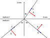Figure 1 Coordinate axes for the present work. The plane of incidence is the plane XZ. The Y-axis points inside the plane of the paper. The interface is the plane XY. The wavevectors are shown in blue. The vectors corresponding to the electric fields for the “p” case are shown in red.

It should be noted that there are no major differences in the procedures developed in references [2–7] for obtaining the formulas and we will not compare them. The only significant (but obvious) detail is to note that the sign of r_|| in textbooks depends on the convention chosen for the positive direction of the reflected electric field [8]. It is evident that the geometrical procedure outlined above for the derivation of the Fresnel formulas is not applicable in two specific situations: (i) internal reflection beyond the critical angle, and (ii) when the second medium is absorbing. These cases are often not covered in detail in most textbooks, which instead refer the reader to the work of [2] for a more rigorous treatment. In this reference, the approach involves using the incident angle θ_i with Snell’s law in its “complex” form to determine the transmitted angle θ_t. This value is then substituted into equations (1)–(4) for further analysis.

Introducing a complex angle for the refracted wave challenges the previous demonstration based on the geometrical projection of fields associated with homogeneous plane waves. Consequently, the physical explanation of the phenomenon must be supplemented to ensure that the practical interpretation of equations (1)–(4) becomes intuitive and clear. The question is analyzed in detail in [9]. Basically two mathematical procedures for addressing the general isotropic interface are compared there: the so called “phase and attenuation” vector representation and the “complex angle” notation. Since these procedures are mathematically complete and well-suited for the problem, we do not intend to repeat them here. The general derivation of the Fresnel coefficients (with specific notation) and a particular numerical example are also developed there. Rather, our goal is to help understanding the use of the complex angle notation since, as the author literally points out in the text of [9], that method “severely lacks in terms of physical interpretability”.

We propose a comprehensive procedure for applying equations (1)–(4) for the transparent-absorbing isotropic interface at any incidence angle, offering a complete interpretation of the resulting practical outcomes. In addition to determining and explicitly writing the amplitudes and phases of all coexisting electric fields, we will illustrate the physical effects introduced by the phase differences in the fields of the reflected and transmitted waves. For the cases where the transmitted wave becomes inhomogeneous, we will also give its propagation direction and penetration decay rate. Finally, although our analysis is limited to the monochromatic case, we believe this work serves as a valuable resource at the undergraduate and graduate levels, as well as for researchers and professionals.

The structure of the paper is as follows. First, we review the application of the Fresnel formulas to the most general case of an isotropic interface, assuming a transparent incident medium, and explicitly compute the Cartesian components of the electric fields of the waves. We examine the specific case of incidence above the critical angle, illustrating the behavior of the electric fields at the interface. Finally, we address incidence on an absorbing substrate, again highlighting the interplay between the various electric fields. For completeness, detailed explanations of the nature of inhomogeneous and evanescent waves are provided in Appendix.

2 Application of the Fresnel formulas in the general plane isotropic interface

The classical analysis of light incidence on a plane interface results in the well-known Fresnel equations (1)–(4). The detailed derivation begins with defining the coordinate axes at the interface. For the “p” case, our Figure 1 aligns with Figure 1 of [10], and also corresponds to the configuration used in [3] to derive equations (1)–(4). The derivation proceeds by enforcing the continuity of the tangential components of the electric and magnetic fields at the interface.

A critical condition for the validity of this approach is that all three waves coexisting at the interface (incident, reflected, and transmitted) must be homogeneous. This phenomenon is particularly well illustrated in Figures 4.53 and 4.54 of [5] which depict external reflection for incidence below and above the Brewster angle, as well as the case of internal reflection.

For instances of internal reflection beyond the critical angle, the classical reference is [2], Section 1.5.4. Since virtually all authors refer to this source, we provide a summary of the method here. Essentially, Snell’s law is first applied to determine the transmitted angle θ_t given the incident angle θ_i, as follows:$$\sin \left({\theta }_t\right)=\frac{n_i\sin \left({\theta }_i\right)}{n_t}=\frac{\sin \left({\theta }_i\right)}{n},\left(n=\frac{n_t}{n_i}\right)\Rightarrow \cos \left({\theta }_t\right)=\pm \sqrt{1-\frac{{\sin }^2\left({\theta }_i\right)}{n^2}}=\pm i\sqrt{\frac{{\sin }^2\left({\theta }_i\right)}{n^2}-1}.$$(5)

Finally, cos(θ_t) is substituted into the previously derived Fresnel equations, followed by a physical interpretation of the resulting waves on an ad hoc basis. Notably, the negative sign is then disregarded, as it pertains to the inhomogeneous wave generated in the second medium.

The case of an absorbing second medium is addressed in [2], Section 14.2. Again, typically textbooks refer to that approach without further considerations, so we summarize the method here. The analysis in [2] begins with the derivation of the wave equation for conducting media, which is then compared to the transparent case. Finally, the transmitted wave is introduced by formally substituting the standard refractive index, dielectric constant, and wavevector with their corresponding complex counterparts. Assuming n_i ≡ 1, the complex refractive index ñ_t = n_t + iκ_t must be used in formulas (1)–(5). While this approach yields correct results – provided the positive sign is chosen in equation (5) – it is not entirely satisfactory in didactical terms and does not fully resolve the physical problem. For example, it does not explicitly address the propagation direction of the inhomogeneous wave in the second medium.

In summary, in the references [2–7], the application of the Fresnel formulas to the general case of an isotropic interface can be effectively carried out using equations (1)–(5). When all three coexisting waves are homogenous, the separate treatment of “s” and “p” polarizations along with the projection of all vectors onto directions parallel and perpendicular to the interface, provides a straightforward and comprehensive approach. This method allows the directions and phases of all amplitudes to be easily determined.

However, when the transmitted wave is evanescent or inhomogeneous, although the separation of “s” and “p” cases remains valid, it becomes necessary to fully describe the reflected and transmitted waves, including their phase delays, propagation directions, and wavelengths, and these topics are not fully addressed in references [2–7]. Furthermore, as pointed out in [9], the use of complex angles in Snell’s law is not comprehensible, although its use has passed on in educational purposes over decades. Here, without duplicating the procedures detailed in [9], we will explain how to use equations (1)–(5) and the physical meaning of the subsequent results. Unfortunately, we cannot make a quick comparison between our procedures and the numerical example developed in [9] for obtaining Figure 3 there, since it corresponds to an interface between two absorbing materials, a configuration that we cannot address. Our developments require a transparent incident medium, while reference [9] imposes no such restriction.

2.1 “s” case

The s-polarized case is simpler than the p-polarized case because all the electric fields oscillate consistently in the same direction (along the Y-axis in Fig. 1). Since our primary focus is on the behavior of the electric fields at the interface, we will omit the s-polarized case and focus exclusively on the p-polarized case. Anyway, the differences in the magnitude and phase of the r_⊥ and t_⊥ coefficients, as well as those associated with the magnetic fields, play a crucial role in determining the behavior of all Poynting vectors. This aspect, however, falls out of the scope of the present work; for further details, refer to [10].

2.2 “p” case

In Figure 1, the positive directions of the electric fields for the validity of equations (1)–(4) are illustrated in red, while the incident, reflected and transmitted wavevectors are shown in blue. The Y-axis that points inside the XZ plane and the magnetic fields (all of them having the Y direction) are not depicted. For the practical application of Fresnel’s formulas, the steps are as follows:

i) computing$$\cos \left({\theta }_t\right)=i\sqrt{\frac{n_i^2\mathrm{si}{\mathrm{n}}^2\left({\theta }_i\right)}{n_t^2}-1},$$(6)ii) computing$$\begin{array}{cc}{r}_{\left|\right|}\equiv \frac{E_r^{\left|\right|}}{E_i^{\left|\right|}}=\frac{n_i\cos {\theta }_t-n_t\cos {\theta }_i}{n_i\cos {\theta }_t+n_t\cos {\theta }_i},& t_{\left|\right|}\equiv \frac{E_t^{\left|\right|}}{E_i^{\left|\right|}}=\frac{2n_i\cos {\theta }_i}{n_i\cos {\theta }_t+n_t\cos {\theta }_i},\end{array}$$(7)iii) computing$$\begin{array}{cc}{t_{\left|\right|}|}_X\equiv \frac{{E_t^{\left|\right|}|}_X}{{E_i^{\left|\right|}|}_X}=t_{\left|\right|}\frac{\cos {\theta }_t}{\cos {\theta }_i},& {t_{\left|\right|}|}_Z\equiv \frac{{E_t^{\left|\right|}|}_Z}{{E_i^{\left|\right|}|}_Z}=t_{\left|\right|}\frac{\sin {\theta }_t}{\sin {\theta }_i}.\end{array}$$(8)

To use equation (8), it is important to note that the two trigonometric quotients are complex quantities. For the reflected beam (see Fig. 1), it is clear that$$\begin{array}{cc}{r_{\left|\right|}|}_X=\frac{{E_r^{\left|\right|}|}_X}{{E_i^{\left|\right|}|}_X}=r_{\left|\right|},& {r_{\left|\right|}|}_Z=\frac{{E_r^{\left|\right|}|}_Z}{{E_i^{\left|\right|}|}_Z}=-r_{\left|\right|}\end{array}.$$(9)

In summary, ${E_i^{\left|\right|}|}_X,{E_i^{\left|\right|}|}_Z,{E_r^{\left|\right|}|}_X,{E_r^{\left|\right|}|}_Z,{E_t^{\left|\right|}|}_X,{E_t^{\left|\right|}|}_Z$ are the complex amplitudes of the waves for the incident, reflected, and transmitted electric fields at the interface for the present “p” case and with the above procedure (summarized by Eqs. (6)–(9)) we are able to specify them.

Indeed, for completeness, we provide here the explicit mathematical expressions for the components of the electric field of the three waves, assuming the incident amplitude to be 1 for simplicity. See Appendix for more details.

Incident field:$${\vec{E}}_i\left(\vec{r}\right)=1\times \exp \left(i{\vec{k}}_i·\vec{r}\right)=\{\begin{array}{c}1\times \cos {\theta }_i\\ 0\\ -1\times \sin {\theta }_i\end{array}\times \exp \left(i{\vec{k}}_i·\vec{r}\right), {\vec{k}}_i=\left(k_i^x, 0, k_i^z\right).$$(10)

Reflected field:$$\begin{array}{ccc}{\vec{E}}_r\left(\vec{r}\right)=\{\begin{array}{c}1\times \cos {\theta }_i\times r_{\left|\right|}\\ 0\\ 1\times \sin {\theta }_i\times r_{\left|\right|}\end{array}\times \exp \left(i{\vec{k}}_r·\vec{r}\right),& {\vec{k}}_r=\left(k_r^x, 0, k_r^z\right), & \mathrm{with} k_r^x\equiv k_i^x,k_r^z\equiv -k_i^z.\end{array}$$(11)

Transmitted field:$$\begin{array}{ccc}{\vec{E}}_t\left(\vec{r}\right)=\{\begin{array}{c}1\times \cos {\theta }_i\times {t_{\left|\right|}|}_X\\ 0\\ -1\times \sin {\theta }_i\times {t_{\left|\right|}|}_Z\end{array}\times \exp \left(i{\vec{k}}_t·\vec{r}\right),& {\vec{k}}_t=\left(k_t^x, 0, k_t^z\right), & \mathrm{with} k_t^x\equiv k_i^x.\end{array}$$(12)

Note that, according to (A.15), $k_t^z$ in equation (12) may be complex-valued.

2.3 Checking the formulas

For this purpose, we compare the results in equations (6)–(9) with those obtained using equations (14) and (15) in [10]. For instance, the first term in (8) $${t_{\left|\right|}|}_X\equiv \frac{{E_t^{\left|\right|}|}_X}{{E_i^{\left|\right|}|}_X}=t_{\left|\right|}\frac{\cos {\theta }_t}{\cos {\theta }_i}=\frac{2n_i\cos {\theta }_i}{n_i\cos {\theta }_t+n_t\cos {\theta }_i}\frac{\cos {\theta }_t}{\cos {\theta }_i}=\frac{2n_i\cos {\theta }_t}{n_i\cos {\theta }_t+n_t\cos {\theta }_i},$$(13)corresponds exactly in [10] to (despite slight differences in notation)$$t_{\left|\right|}^x\equiv \frac{E_t^x}{E_i^x}=\frac{{\epsilon }_i{k}_t^z}{{\epsilon }_t{k}_i^z}{t}_p^y=\frac{{\epsilon }_i{k}_t^z}{{\epsilon }_t{k}_i^z}\frac{2{\epsilon }_t{k}_i^z}{{\epsilon }_t{k}_i^z+{\epsilon }_i{k}_t^z}=\frac{2{\epsilon }_i{k}_t^z}{{\epsilon }_t{k}_i^z+{\epsilon }_i{k}_t^z}.$$(14)

The equality ${t_{\left|\right|}|}_X=t_{\left|\right|}^x$, follows directly from the basic identities (see Appendix for the details):$$\begin{array}{cccc}{\epsilon }_i=n_i^2,& {\epsilon }_t=n_t^2,& k_i^z=k_0{n}_i\cos {\theta }_i& k_t^z=k_0{n}_t\cos {\theta }_t.\end{array}$$(15)

Similarly, the following equivalences can also easily be shown:$$\begin{array}{ccc}{t_{\left|\right|}|}_Z=t_p^z,& {r_{\left|\right|}|}_X=r_p^x,& {r_{\left|\right|}|}_Z=r_p^z.\end{array}$$(16)

In summary, the direct procedure using the complex angle approach (Eqs. (6)–(9)) is equivalent to the more formal developments presented in [10], with the advantage of being more straightforward. Of course, the methods outlined in [9] can also be applied. However, we believe that our approach is faster and, hopefully, more intuitive.

We will now demonstrate how equations (6)–(9) are employed to solve and interpret the general case of an isotropic plane interface, with particular focus on incidence beyond the critical angle and on configurations involving an absorbing second medium. In both cases, additional information about the transmitted wave is required for completeness (see Appendix and [10]).

3 Two examples

We plan to graphically illustrate the behavior of the fields at the interface in two non-trivial cases.

3.1 Internal reflection

Consider the interface between two transparent media with refractive indices n_i = 1.5, n_t = 1.0, with the incidence angle θ_i = 55°. Since the incidence is above the critical angle, we have total reflection. The ratios between tangential and normal components of the electric field are given by the formulas (7)–(9). Here they give, in detail,$$r_P=1.0\times \exp \left[2\pi i\left(\frac{56.34}{360}\right)\right],$$(17) $$\{\begin{array}{c}{t_{\left|\right|}|}_X= t_{\left|\right|}\frac{\cos {\theta }_t}{\cos {\theta }_i}=1.42\times \exp \left[2\pi i\left(\frac{-61.83}{360}\right)\right] \frac{0.71\times \exp \left[2\pi i\right(90/360\left)\right]}{0.573}=1.76\times \exp \left[2\pi i\left(\frac{28.17}{360}\right)\right], \\ {t_{\left|\right|}|}_Z=t_{\left|\right|}\frac{\sin {\theta }_t}{\sin {\theta }_i}=1.42\times \exp \left[2\pi i\left(\frac{-61.83}{360}\right)\right]\frac{1.23}{0.82}=2.12\times \exp \left[2\pi i\left(\frac{-61.83}{360}\right)\right]. \end{array}$$

Since the phases of $r_{\left|\right|}, {t_{\left|\right|}|}_X, {t_{\left|\right|}|}_Z$ are not 0° or 180°, the complex amplitudes for the reflected and transmitted waves are neither in phase nor opposite with respect to the incident one. In fact, the three complex quantities $r_{\left|\right|}, {t_{\left|\right|}|}_X, {t_{\left|\right|}|}_Z$ have been expressed with phase angles in degrees in the argument of the complex exponential, clearly illustrating the differences relative to the incident wave.

Figure 2 shows a snapshot of the relevant vectors at the origin of the coordinate system at the instant when the incident electric field (${\vec{E}}_i\left(0\right)$) reaches its maximum. The coordinate axes are the same as for Figure 1, but now only the interface is depicted (as a horizontal line), with its normal direction represented by a dotted line for clarity. The directions of the incident, reflected, and transmitted waves are shown in blue. While these vectors are plotted slightly apart for visual clarity, it should be noted that all electric field vectors (displayed in red) correspond to a common point: the origin of the coordinates system. According to equation (17), the amplitude of the reflected electric field equals that of the incident field. However, since the reflected field is not in phase with the incident field at its maximum, the length of the reflected E-vector appears shorter. The fields ${\vec{E}}_i\left(0\right),{\vec{E}}_r\left(0\right),{\vec{E}}_t\left(0\right),{\vec{E}}_i\left(0\right)+{\vec{E}}_r\left(0\right)$ are shown. It can be observed that the tangential (horizontal) component of the electric field (the X-coordinate of the ${\vec{E}}_t\left(0\right),{\vec{E}}_i\left(0\right)+{\vec{E}}_r\left(0\right)$ vectors) remains continuous across the interface between the two media, while the normal component (their Z-coordinate) exhibits discontinuity.

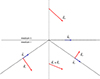Figure 2 Electric fields (in red) at the origin of the coordinate axes. We see (although shown apart) the vectors ${\vec{E}}_i\left(0\right),{\vec{E}}_r\left(0\right),{\vec{E}}_t\left(0\right),{\vec{E}}_i\left(0\right)+{\vec{E}}_r\left(0\right)$ corresponding to the exact time where the incident (${\vec{E}}_i\left(0\right)$) field is maximum. The wavevectors are also shown in blue.

It is worth noting that, unlike the case of a transparent interface below the critical angle, the incident and reflected electric fields here are neither in phase nor in opposite phase. Consequently, Figure 2 provides valuable insight into the not-intuitive behavior of the fields at the interface.

Figure 3 illustrates the same electric fields as shown in Figure 2, along with the electric fields at a moment 1/18 of a time period later. Comparing the two figures reveals that the incident and reflected electric fields of the homogeneous transverse waves in medium “i” are both smaller, leading to a total electric field that rotates clockwise in the X-Z plane. Similarly, in medium “t”, the electric field increases in magnitude, with its vector rotating also clockwise in Figure 3. For illustration, the dots forming ellipses represent the trajectories of the tips of the total electric field vectors in media “i” and “t” over a full period of the wave. As in Figure 2, we observe that the tangential components of the electric fields in medium “i” and medium “t” remain continuous across the interface, with their horizontal projections aligning perfectly. In contrast, the normal components exhibit discontinuity.

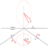Figure 3 Electric fields (in red) at the origin of the coordinate axes for two different instants of time. First, for the same time as in Figure 2 and, second, for the time T/18 later (being T the time period). Thus, we see that both ${\vec{E}}_i\left(0\right),{\vec{E}}_r\left(0\right)$ get shorter, making ${\vec{E}}_i\left(0\right)+{\vec{E}}_r\left(0\right)$ to turn clockwise. Similarly, ${\vec{E}}_t\left(0\right)$ gets shorter and turns counterclockwise. The red dots show the tips of the electric fields for a full time period T.

Despite this detailed depiction, critical information about the transmitted wave remains missing – specifically, its decay rate. Using equation (55) from Section 1.5.4 of [2], the real exponential term governing the in-depth decay of the electric field is given by:$$\exp \left(-\frac{\omega z}{v_2}\sqrt{\frac{\mathrm{si}{\mathrm{n}}^2{\theta }_i}{n^2}-1}\right)=\exp \left(-2\pi \frac{z}{{\lambda }_2}\sqrt{\frac{\mathrm{si}{\mathrm{n}}^2{\theta }_i}{n^2}-1}\right).$$(19)

Since v₂ and λ₂ represent the speed and wavelength in the second medium, the final expression in (19) (as indicated in [2]) suggests that “the amplitude decreases very rapidly … the effective depth of penetration being … of the order of a wavelength”. However, this statement is somewhat misleading, as when the incidence angle is θ_i = 55° (for n_i = 1.5, n_t = 1.0, i.e., n = 1.0/1.5), the ratio $\left(\frac{z}{{\lambda }_2}\right)$ in the exponent is multiplied by $2\pi \sqrt{\frac{\mathrm{si}{\mathrm{n}}^2{\theta }_i}{n^2}-1}\approx 4.49$. However, if the incidence angle were θ_i = 41.9° (the critical angle being θ_C = 41.8°), we would obtain the following factor multiplying inside the exponential:$$2\pi \sqrt{\frac{\mathrm{si}{\mathrm{n}}^2{\theta }_i}{n^2}-1}\approx 0.37.$$(20)

This result shows that the penetration depth at an incidence of 41.9° is more than an order of magnitude greater than at 55°. In fact, it is evident that the value given by expression (20) approaches zero as the incidence angle nears the critical value θ_i → θ_C = 41.8°. Thus, it is not entirely accurate to say that evanescent waves always decay rapidly, as their decay rate is highly sensitive to the incidence angle.

3.2 Absorbing substrate

As a second example for illustrating the behavior of the fields, consider an interface between two media with refractive indices n_i = 1.0, n_t = 0.46 + 3.13 i (corresponding approximately to brass), and an incidence angle of θ_i = 40°. Using equations (6)–(9), we find:$$r_{\left|\right|}=0.897\times \exp \left[2\pi i\left(\frac{-134.7}{360}\right)\right],$$(21) $$\{\begin{array}{c}{t_{\left|\right|}|}_X=t_{\left|\right|}\frac{\cos {\theta }_t}{\cos {\theta }_i}=0.55\times \exp \left[2\pi i\left(\frac{-60.28}{360}\right)\right]\frac{1.02\times \exp \left[2\pi i(0.33/360) \right]}{0.766}=0.737\times \exp \left[2\pi i\left(\frac{-59.95}{360}\right)\right],\\ {t_{\left|\right|}|}_Z=t_{\left|\right|}\frac{\sin {\theta }_t}{\sin {\theta }_i}=0.55\times \exp \left[2\pi i\left(\frac{-60.28}{360}\right)\right]\frac{0.20\times \exp \left[2\pi i(-81.6/360)\right]}{0.643}=0.175\times \exp \left[2\pi i\left(\frac{-141.9}{360}\right)\right].\end{array}$$(22)

The phases in (21)–(22) are neither 0° nor 180°. As before, the detailed calculations for the three complex quantities $r_{\left|\right|},{t_{\left|\right|}|}_X,{t_{\left|\right|}|}_Z$ have been expressed with phase angles written in degrees in the argument of the complex exponentials.

Figure 4 depicts a snapshot at the instant when the incident electric field reaches its maximum. Figure 4 illustrates the incident and reflected electric fields, along with the resulting electric field in medium “i” and the transmitted electric field. As before in Figure 3, the dots correspond to the tips of the electric field vectors over a full time period.

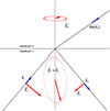Figure 4 Electric fields (in red) at the origin of the coordinate axes, as in Figure 2. We see (shown separately) the vectors ${\vec{E}}_i\left(0\right),{\vec{E}}_r\left(0\right),{\vec{E}}_t\left(0\right),{\vec{E}}_i\left(0\right)+{\vec{E}}_r\left(0\right)$ corresponding to the exact time where the incident (${\vec{E}}_i\left(0\right)$) field is maximum. The red dots show the tips of the electric fields for a full time period T. In contrast with Figure 3, now the ellipse in medium “i” is described counterclockwise, while the ellipse in medium “t” rotates clockwise.

We could demonstrate now that the ellipse in medium “i” is described rotating counterclockwise, while the ellipse in medium “t” is turned clockwise. As expected from basic theory, the tangential component of the electric field remains continuous across the interface, whereas the normal component does not. It is important to note that in this case, where the second medium is absorbing, the wave in medium “t” is inhomogeneous and not purely transverse [11, 12]. The direction of phase propagation in medium “t” is indicated and labeled as $\mathrm{Re}\left({\vec{k}}_t\right)$. The decay rate would correspond to $\mathrm{Im}\left({\vec{k}}_t\right)$, a vector oriented in the upward normal direction. To fully characterize the inhomogeneous transmitted wave, three key parameters are required: (i) the direction of phase propagation, (ii) the wavelength, and (iii) the rate of decay of the wave (as we define by (19)). The theoretical framework for these calculations is provided in [10], while the numerical procedures are elaborated upon in Appendix.

The computed results, assuming λ_i = 587.0 nm, are the following:$$\begin{array}{cc}{\theta }_t=54.96\mathrm{°},& \left(\mathrm{from} (\mathrm{A}.17)\right),\end{array}$$(23) $$\begin{array}{cc}{\lambda }_t=747.7 \mathrm{nm},& \left(\mathrm{from} (\mathrm{A}.16)\right), \end{array}$$(24) $$\begin{array}{cc}\exp \left(-0.714\frac{z}{{\lambda }_t}\right)& \left(\mathrm{from} (\mathrm{A}.15)\right).\end{array}$$(25)

4 Summary and conclusions

We have shown how Fresnel formulas can be applied to a general isotropic interface (transparent incident medium and absorbing second medium) by employing our equations (8)–(12), which conveniently represent the fields within a unified coordinate system.

For less intuitive cases where the transmitted wave is inhomogeneous, we provide visual illustrations to highlight the physical significance of phase delays between coexisting electric fields. Additionally, our approach offers practical methods for determining the exponential decay rate, wavelength, and propagation direction, as outlined in equations (A.15)–(A.17) of Appendix. This includes the special case of evanescent waves.

In summary, the procedure presented here for determining the electric fields at the interface is more practical and efficient than previously established formal methods [9, 10]. Moreover, it highlights the underlying physics of the fields at the interface while addressing critical properties of light in the second medium, such as its propagation direction and penetration depth.

Funding

This work was supported by projects TED2021-129639B-I00, CNS2022-136051 and PID2022-138699OB-I00 from the Ministerio de Ciencia e Innovación of Spain. Work also supported by TED2021-129639B-I00/AEI/10.13039/501100011033/Unión Europea NextGenerationEU/PRTR

Conflicts of interest

The authors do not have any kind of conflict of interest.

Data availability statement

This article has no associated data generated and/or analyzed.

Author contribution statement

The first author is responsible for formulating the original idea, while the second author contributed essential comments that are reflected in the final text.

References

Appendix

We summarize the properties of inhomogeneous plane waves that are relevant for the present paper.

Inhomogeneous versus homogeneous plane waves

What are monochromatic inhomogeneous plane waves? What is their physical significance? First, remember that monochromaticity for an electromagnetic field means that the space $\left(\vec{r}\right)$ and time (t) variations can be factorized in the form$$\mathrm{physical\_field}=\mathrm{Re}\left[\vec{E}(\vec{r},t)\right]=\mathrm{Re}\left[\vec{E}\left(\vec{r}\right)\exp (-\mathrm{i\omega }t)\right]$$(A.1)where ω is the angular frequency and $\vec{E}\left(\vec{r}\right)$ is a 3-D vector with (in the most general case) complex components $\vec{E}\left(\vec{r}\right)=\left(E^x\left(\vec{r}\right),E^y\left(\vec{r}\right),E^z\left(\vec{r}\right)\right)$.

Linear operations on the fields (addition, derivation…) will not mix real and imaginary parts of the complex expressions and, therefore, complex form will always be used in our work for convenience. Specifically, we will only focus on $\vec{E}\left(\vec{r}\right)$ as it contains all the significant information.

In 3-D space, a particular case of (A.1) above is the monochromatic homogeneous plane wave inside a transparent medium with refractive index n. It may be simply written in terms of the scalar product between a standard wavevector $\vec{k}=\left(k^x,k^y,k^z\right)$ and the position vector $\vec{r}$. The vector $\vec{k}$ has three real-valued components, points in the direction of the wave propagation and is related to the wavelength by $\lambda =2\pi \vec{k}$. Thus, the monochromatic homogeneous plane wave is written$$\vec{E}\left(\vec{r},t\right)={\vec{E}}_0\exp i\left(\vec{k}\cdot \vec{r}-\omega t\right),$$(A.2)where ${\vec{E}}_0$ is a constant vector with three complex components. Since all the relevant information on the wave is contained in the spatial part$$\vec{E}\left(\vec{r}\right)={\vec{E}}_0\exp \left(i\vec{k}\cdot \vec{r}\right),$$(A.3)we conclude that the couple of vectors ${\vec{E}}_0$ and $\vec{k}$ fully define our homogeneous monochromatic plane wave.

Now consider not just one but two standard vectors, namely $\overrightarrow{k_{\mathfrak{R}}},\overrightarrow{k_{\mathfrak{I}}}$, each with three real components (thus each one indicating one direction in 3-D space), and consider the following mathematical expression$$\vec{k}\equiv \overrightarrow{k_{\mathfrak{R}}}+i \overrightarrow{k_{\mathfrak{I}}},$$(A.4)as the definition of the complex wavevector $\vec{k}$ and, for the electric field, consider the expression$$\vec{E}\left(\vec{r}\right)={\vec{E}}_0\exp \left(i\vec{k}·\vec{r}\right)={\vec{E}}_0\exp i\left(\left(\overrightarrow{k_{\mathfrak{R}}}+i \overrightarrow{k_{\mathfrak{I}}}\right)·\vec{r}\right)=\left(\exp \left(-\overrightarrow{k_{\mathfrak{I}}}·\vec{r}\right){\vec{E}}_0\right)\exp \left(i\overrightarrow{k_{\mathfrak{R}}}·\vec{r}\right).$$(A.5)

The phase variations due to $\exp (i\overrightarrow{k_{\mathfrak{R}}}·\vec{r})$ are the same as for a homogeneous wave with wavevector $\overrightarrow{k_{\mathfrak{R}}}$. The constant amplitude term (${\vec{E}}_0$) also appears in (A.5) as before in (A.3), but now in (A.5) is multiplied by a real exponential term given by $\exp (-\overrightarrow{k_{\mathfrak{I}}}·\vec{r})$. Therefore, by introducing the complex wavevector (A.4) we have defined an inhomogeneous monochromatic wave given by expression (A.5). In other words, an inhomogeneous plane wave is defined by the set of the three vectors ${\vec{E}}_0, \overrightarrow{k_{\mathfrak{R}}}, \overrightarrow{k_{\mathfrak{I}}}$ (i.e. ${\vec{E}}_0,\mathrm{Re}\left(\vec{k}\right) \mathrm{and} \mathrm{Im}\left(\vec{k}\right)$) instead of the two vectors ${\vec{E}}_0$ and $\vec{k}$ which defined a homogeneous plane wave.

When we study plane waves at an interface (within the monochromatic assumption) the calculation of the couples of values ${\vec{E}}_0$ and $\vec{k}$ or sets of three values ${\vec{E}}_0,\mathrm{Re}\left(\vec{k}\right) \mathrm{and} \mathrm{Im}\left(\vec{k}\right)$ that define the three coexisting waves (incident, reflected, and transmitted), fully solves the physical problem. Indeed, to directly know the instantaneous values of all the fields, it is only necessary to use (A.3) together with (A.1) for each wave.

Wave equation in isotropic absorbing materials

According to Maxwell equations, the wave equation for the spatial part of the electric field in an isotropic medium with relative magnetic permittivity μ and complex refractive index $\tilde{n}=n+\mathrm{i\kappa }$ (or complex generalized permittivity ε, with με = (n + iκ)²), is:$$\Delta \vec{E}\left(\vec{r}\right)+\mu \epsilon {\left(\frac{\omega }{c}\right)}^2\vec{E}\left(\vec{r}\right)=0.$$(A.6)

The same equation is valid for the magnetic field. It is straightforward to check that the monochromatic inhomogeneous plane waves in the form$$\vec{E}\left(\vec{r}\right)={\vec{E}}_0\exp \left(i\vec{k}\cdot \vec{r}\right),$$(A.7)with $\vec{k}=\mathrm{Re}\left(\vec{k}\right)+i\mathrm{Im}\left(\vec{k}\right)$, fulfill this equation provided that$$\begin{array}{cc}\vec{k}\cdot {\vec{E}}_0=0,& \vec{k}\cdot {\vec{H}}_0=0,\end{array}$$(A.8) $${\left(\vec{k}\right)}^2=\vec{k}\cdot \vec{k}={\left(k^x\right)}^2+{\left(k^y\right)}^2+{\left(k^z\right)}^2=\mu \epsilon \frac{{\omega }^2}{c^2}=\mu \epsilon k_0^2=P+\mathrm{iQ}=C \left(C\in \mathbb{C};P,Q\in \mathbb{R}\right), \left(\frac{\omega }{c}=k_0\right).$$(A.9)

Equation (A.9) is the dispersion equation. Note that this dispersion equation does not contain the quantity ${\left|\vec{k}\right|}^2=\vec{k}\cdot {\vec{k}}^{\mathrm{*}}(\in \mathbb{R})$ but the value ${\left(\vec{k}\right)}^2=\vec{k}\cdot \vec{k}=\mu \epsilon k_0^2(\in \mathbb{C})$ instead. The condition (A.9) on $\vec{k}=\mathrm{Re}\left(\vec{k}\right)+i\mathrm{Im}\left(\vec{k}\right)$ implies:

• $${\left|\mathrm{Re}\left(\vec{k}\right)\right|}^2-{\left|\mathrm{Im}\left(\vec{k}\right)\right|}^2=k_0^2\left(n^2-{\kappa }^2\right)=P (\in \mathbb{R})$$(A.10) in words, the difference between the square modulus of the real part of $\vec{k}$ and the imaginary part of $\vec{k}$ is constant.

• $$\left|\mathrm{Re}\left(\vec{k}\right)\right|\left|\mathrm{Im}\left(\vec{k}\right)\right|\cos \left(\phi \right)=k_0^2\mathrm{n\kappa }=Q \left(\in \mathbb{R}\right),$$(A.11) i.e., the dot product between vector $\mathrm{Re}\left(\vec{k}\right)$ and vector $\mathrm{Im}\left(\vec{k}\right)$ is constant.

Evanescent waves

One particular case will also be relevant for us. When the medium is transparent (κ = 0), the wave equation (A.6) still allows inhomogeneous waves as a specific solution: according to expression (A.11) it is only necessary that cos(φ) = 0, i.e., $\mathrm{Re}\left(\vec{k}\right)\perp \mathrm{Im}\left(\vec{k}\right)$. This kind of inhomogeneous waves are the well-known “evanescent” waves.

In summary, the wave equation in absorbing materials leads to two conditions (A.10) and (A.11) to be fulfilled by the three real-valued quantities $\left|\mathrm{Re}\left(\vec{k}\right)\right|,\left|\mathrm{Im}\left(\vec{k}\right)\right|$ and the angle φ. It is important to grasp the physical meaning of the results we have just obtained: inside an absorbing medium, the complex expressions (A.7), with the restrictions (A.8)–(A.11), represent an electromagnetic field that fulfills the Maxwell equations in the medium. This means that the real physical fields given by (A.3) and (A.1) are valid solutions of Maxwell equations, that we name inhomogeneous plane waves since the phase propagates like a plane wave in one direction (defined by $\mathrm{Re}\left(\vec{k}\right)$) while decays in another direction (defined by $\mathrm{Im}\left(\vec{k}\right)$). As a particular case, the results applied to transparent media explain the existence of evanescent waves.

Plane waves reflected and refracted at an interface: computing the wavevectors

Consider the coordinate axes given by Figure 1. The interface is the (X-Y) plane and the plane of incidence is the (X-Z) plane. Dealing only with isotropic materials, the symmetry of the configuration guarantees that the incident, reflected and transmitted wavevectors remain in the X-Z plane. Since the emergent medium is (in our general case) absorbing, we will assume an inhomogeneous wave there. Due to the isotropy of the materials and the symmetry of the configuration, the direction of the vector $\mathrm{Im}\left(\vec{k}\right)$ which represents the direction of the decay of the transmitted wave (if decay exists), has to point in the direction of our positive Z-axis.

For the two media, incident (“i”) and transmitted (“t”), assume that the optical constants are, respectively,$$\begin{array}{cc}i: n_i^2={\epsilon }_i,{\mu }_i\equiv 1 \left(\mathrm{all}\in \mathbb{R}\right);& t:{\left(n_t+i{\kappa }_t\right)}^2={\epsilon }_t\left(\in \mathbb{C}\right),{\mu }_t\equiv 1 \left(\in \mathbb{R}\right)\end{array}$$(A.12)

For an incidence angle θ in the incidence plane (X-Z), we need to calculate the two components (X and Z) of all the wavevectors (all of them have no Y component). This can be done by taking into account that their tangential components (here the X coordinates) have to be the same for the incident, reflected, and transmitted wavevectors.

There are three plane waves in contact at the interface: the incident and reflected ones contained in medium “i” (with refractive index n_i) and with wavevectors $(k_i^x,0,k_i^z)$ and $(k_r^x,0,k_r^z)$ respectively, and the transmitted wave inside medium “t” (with index n_t + iκ_t), and with wavevector $(k_t^x,0,k_t^z)$. Because of the equality of the X components of all the wavevectors, using the same notation as in [10] we will write all the X components of all the wavevectors in terms of the X component of the incident wavevector $k_i^x$:$$\begin{array}{ccccc}{\vec{k}}_i=\left(k_i^x,0,k_i^z\right),& {\vec{k}}_r=\left(k_i^x,0,k_r^z\right),& {\vec{k}}_t=\left(k_i^x,0,k_t^z\right),& k_i^x,k_i^z,k_r^z\in \mathbb{R},& k_t^z\in \mathbb{C}\end{array}.$$(A.13)

Thus, for the “i” medium we have$$\begin{array}{cc}{k}_i^x=k_r^x=k_0{n}_i\sin \left(\theta \right),& k_i^z=-k_r^z=\sqrt{{\left(k_0{n}_i\right)}^2-{\left(k_i^x\right)}^2}\left(\in \mathbb{R}\right).\end{array}$$(A.14)

For finding the Z component in medium “t” we have to use the algebraic formula for the complex square root in (A.9) $$k_t^z=\sqrt{{\left(k_0\left(n_t+i{\kappa }_t\right)\right)}^2-{\left(k_i^x\right)}^2}=\mathrm{Re}\left(k_t^z\right)+i\mathrm{Im}\left(k_t^z\right)=k_0\left(\sqrt{\frac{A+B}{2}}+i\sqrt{\frac{B-A}{2}}\right),\{\begin{array}{c}A=n_t^2-{\kappa }_t^2-n_i^2\mathrm{si}{\mathrm{n}}^2\left(\theta \right)\\ B=\sqrt{A^2+{\left(2n_t{\kappa }_t\right)}^2}\end{array}.$$(A.15)

Finally, the wavelength λ_t is obtained from$$\left|\mathrm{Re}\left({\vec{k}}_t\right)\right|=\sqrt{{\left(k_i^x\right)}^2+{\left(\mathrm{Re}\left(k_t^z\right)\right)}^2}=\frac{2\pi }{{\lambda }_t}$$(A.16)and the propagation angle in medium “t” is$$\phi ={\tan }^{-1}\left(\frac{k_i^x}{\mathrm{Re}\left(k_t^z\right)}\right).$$(A.17)

Since the value λ_t in medium “t” (defined as the distance for the periodicity of the phase) is found from (A.16), this wavelength changes with the incidence angle and it is not a fixed quantity depending only on the refractive index of medium “t”, like for transparent materials.

The procedure for computing $k_t^z$ given by (A.15) is very convenient since is general and automatically gives the complete answer: if $\mathrm{Im}\left(k_t^z\right)=0$ (since $\mathrm{Im}\left({\vec{k}}_t\right)$ has only Z component as explained) it means that $\mathrm{Im}\left({\vec{k}}_t\right)\equiv 0$ and the transmitted wave is homogeneous. Besides, the value of angle φ is also obtained from (A.17), including evanescent waves as particular case.

Thus, for all practical isotropic interfaces from a transparent medium “i” to any material in medium “t”, with the above procedure summarized in equations (A.13)–(A.17) we will know all the wavevectors for the waves, besides the incident one $\left({\vec{k}}_i\right)$. For the transmitted wave $\mathrm{Re}\left({\vec{k}}_t\right)$ defines the wavelength and propagation direction and $\mathrm{Im}\left({\vec{k}}_t\right)$ represents the decay of the transmitted inhomogeneous wave.

All Figures

	Figure 1 Coordinate axes for the present work. The plane of incidence is the plane XZ. The Y-axis points inside the plane of the paper. The interface is the plane XY. The wavevectors are shown in blue. The vectors corresponding to the electric fields for the “p” case are shown in red.
In the text

	Figure 2 Electric fields (in red) at the origin of the coordinate axes. We see (although shown apart) the vectors ${\vec{E}}_i\left(0\right),{\vec{E}}_r\left(0\right),{\vec{E}}_t\left(0\right),{\vec{E}}_i\left(0\right)+{\vec{E}}_r\left(0\right)$ corresponding to the exact time where the incident (${\vec{E}}_i\left(0\right)$) field is maximum. The wavevectors are also shown in blue.
In the text

Figure 3 Electric fields (in red) at the origin of the coordinate axes for two different instants of time. First, for the same time as in Figure 2 and, second, for the time T/18 later (being T the time period). Thus, we see that both ${\vec{E}}_i\left(0\right),{\vec{E}}_r\left(0\right)$ get shorter, making ${\vec{E}}_i\left(0\right)+{\vec{E}}_r\left(0\right)$ to turn clockwise. Similarly, ${\vec{E}}_t\left(0\right)$ gets shorter and turns counterclockwise. The red dots show the tips of the electric fields for a full time period T.

In the text

Figure 4 Electric fields (in red) at the origin of the coordinate axes, as in Figure 2. We see (shown separately) the vectors ${\vec{E}}_i\left(0\right),{\vec{E}}_r\left(0\right),{\vec{E}}_t\left(0\right),{\vec{E}}_i\left(0\right)+{\vec{E}}_r\left(0\right)$ corresponding to the exact time where the incident (${\vec{E}}_i\left(0\right)$) field is maximum. The red dots show the tips of the electric fields for a full time period T. In contrast with Figure 3, now the ellipse in medium “i” is described counterclockwise, while the ellipse in medium “t” rotates clockwise.

In the text

References

- Fresnel A, Mémoire sur la Loi des modifications que la réflexion imprime à la lumière polarisée (read at Academie des Sciences, 7 January 1823). [Google Scholar]
- Born M, Wolf E, Principles of Optics: Electromagnetic Theory of Propagation, Interference and Diffraction of Light, 7th edn (Cambridge University Press, 1999). ISBN: 9781139644181. [CrossRef] [Google Scholar]
- Fowles GR, Introduction to Modern Optics (Dover Publications Inc, New York, 1975). [Google Scholar]
- Novotny L, Hecht B, Principles of Nano-Optics (Cambridge University Press, 2012). Online ISBN: 9780511794193. [CrossRef] [Google Scholar]
- Hecht E, Optics, 5th edn (Pearson, Boston, 2017). [Google Scholar]
- Peatross J, Ware M, Physics of Light and Optics, 2015 edn (Department of Physics, Brigham Young University, Provo, Utah, 2016). Available at https://optics.byu.edu. [Google Scholar]
- Cabrera JM, López FJ, Agulló-López F, Optica Electromagnética Vol. 1. Fundamentos, 1st edn. (Pearson Addison-Wesley, 1998). ISBN: 97884782902157. [Google Scholar]
- Arteaga O, Bosch S, The π phase in polarization optics: a retrospective, J. Opt. Soc. Am. A 42, 327 (2025). [Google Scholar]
- Schake MC, Comparison of recent results for the determination of effective propagation constants at attenuating interfaces, Eur. J. Phys. 39, 015302 (2018). [Google Scholar]
- Bosch S, Ferré-Borrull J, Sancho-Parramon J, Arteaga O, Compact formulation of the transparent-absorbing isotropic interface electromagnetic problem, J. Opt. Soc. Am. A 39, 1774 (2022). [Google Scholar]
- Halevi P, Plane electromagnetic waves in material media: are they transverse waves?, Am. J. Phys. 48, 861 (1980). [Google Scholar]
- Halevi P, Mendoza-Hernández A, Temporal and spatial behavior of the Poynting vector in dissipative media: refraction from vacuum into a medium, J. Opt. Soc. Am. A 71, 1238 (1981). [Google Scholar]